Choosing a grid

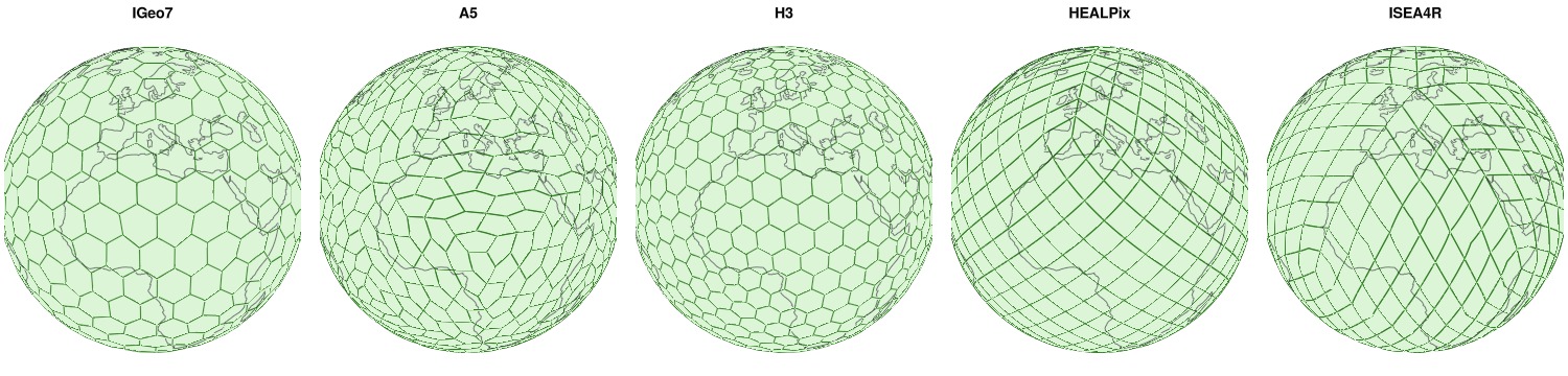
A discrete global grid system divides the sphere into cells at several resolutions. Choose a system for its cell geometry and compatibility with your data, then choose a level for the cell size you need.

This tutorial compares the global systems, finds a level from a size in metres, and checks the coordinate convention used to locate cells. The globes above show cells roughly 800 km across. This tutorial compares five systems; the DGGS gallery shows the supported global systems.

import DiscreteGlobalGrids as DGG
import GeometryOps as GO
using Statistics

Choose a cell geometry

Start with the requirements of your analysis:

System	Cell shape	Useful when you need
IGeo7	Hexagons, with twelve pentagons	Hexagonal neighbourhoods and approximately equal cell areas
H3	Hexagons, with twelve pentagons	Compatibility with existing H3 identifiers and datasets
A5	Pentagons	A single cell shape with nearly equal areas
HEALPix	Curved quadrilaterals	Equal-area cells and compatibility with HEALPix maps
ISEA4R	Rhombi	Equal-area cells with four edge neighbours

H3 supports native H3 identifiers. HEALPix supports nested and ring index conversion; reorder values when changing pixel order. ISEA4R numbering is package-defined; compatibility with external ISEA4R identifiers is not established.

Compare physical resolution

Cell shape affects neighbourhood calculations. Cell area affects the weights needed for spatial averages. We examine both below.

Compare resolutions by cell size: each system assigns its own meaning to a level number. Approximate cell widths in kilometres are:

level	IGeo7	A5	H3	HEALPix	ISEA4R
0	6520 km	6524 km	2026 km	6520 km	7142 km
1	2721 km	2917 km	776 km	3260 km	3571 km
2	1021 km	1459 km	298 km	1630 km	1786 km
3	386 km	729 km	113 km	815 km	893 km
4	146 km	365 km	43 km	408 km	446 km
5	55 km	182 km	16 km	204 km	223 km
6	21 km	91 km	6 km	102 km	112 km
7	8 km	46 km	2 km	51 km	56 km
8	3 km	23 km	0.9 km	25 km	28 km
9	1 km	11 km	0.3 km	13 km	14 km
10	0.4 km	6 km	0.1 km	6 km	7 km

Find the level for a cell size

cellsize(sys, level) is the typical cell width in metres, the side of a square with the median cell's area:

DGG.cellsize(DGG.IGeo7System(), 5)

55089.48974970403

Use levelfor to choose the closest available level. It accepts a size in metres, a raster, or another grid:

DGG.levelfor(DGG.IGeo7System(), 25_000)

6

Cell width shrinks by √7 per level on IGeo7 and H3 and by 2 on A5, HEALPix and ISEA4R, so levelfor returns the level nearest in ratio.

Count a cell's neighbours

Neighbourhood algorithms need a rule for which cells to include. Edge() includes cells sharing an edge; Vertex() also includes cells that touch at a corner. On a hexagonal grid these usually give the same neighbours. Quadrilateral grids distinguish the two, much like a raster's four- and eight-neighbour rules. Distances between centres depend on the grid geometry.

Compare the two rules at Zürich:

igeo7 = DGG.levelgrid(DGG.IGeo7System(), 4)
zurich = DGG.cellat(igeo7, 8.5, 47.4)
(DGG.neighborcount(igeo7, zurich; connectivity = DGG.Edge()),
 DGG.neighborcount(igeo7, zurich; connectivity = DGG.Vertex()))

(6, 6)

healpix = DGG.levelgrid(DGG.HEALPixSystem(), 4)
diamond = DGG.cellat(healpix, 8.5, 47.4)
(DGG.neighborcount(healpix, diamond; connectivity = DGG.Edge()),
 DGG.neighborcount(healpix, diamond; connectivity = DGG.Vertex()))

(4, 8)

Twelve cells at every level of IGeo7 and H3 are pentagons, one at each vertex of the icosahedron. A kernel that assumes six neighbours has to handle those twelve; neighborcount returns 5 there.

count(c -> DGG.neighborcount(igeo7, c; connectivity = DGG.Edge()) == 5,
      DGG.CellVector(igeo7))

12

Measure how equal the cell areas are

Equal-area cells let you compute an area mean with an ordinary mean. For unequal cells, weight values by cell_area.

Compare the largest and smallest cell areas at a resolution near 500 km. A ratio of 1 means equal areas. The middle-90% ratio shows the spread after excluding the smallest and largest 5% of cells:

map([DGG.IGeo7System(), DGG.A5System(), DGG.H3System(),
     DGG.HEALPixSystem(), DGG.ISEA4RSystem()]) do sys
    grid = DGG.levelgrid(sys, DGG.levelfor(sys, 500_000))
    areas = [DGG.cell_area(grid, c) for c in DGG.CellVector(grid)]
    lo, hi = quantile(areas, (0.05, 0.95))
    (; system = nameof(typeof(sys)),
       whole_level = round(maximum(areas) / minimum(areas); digits = 2),
       middle_90 = round(hi / lo; digits = 2))
end

5-element Vector{@NamedTuple{system::Symbol, whole_level::Float64, middle_90::Float64}}:
 (system = :IGeo7System, whole_level = 1.39, middle_90 = 1.02)
 (system = :A5System, whole_level = 1.01, middle_90 = 1.01)
 (system = :H3System, whole_level = 2.22, middle_90 = 1.58)
 (system = :HEALPixSystem, whole_level = 1.0, middle_90 = 1.0)
 (system = :ISEA4RSystem, whole_level = 1.0, middle_90 = 1.0)

HEALPix and ISEA4R have equal areas by construction. A5 and most IGeo7 cells have similar areas, while IGeo7's pentagons are smaller. H3 has a larger spread. Use area weights whenever those differences matter to your statistic, including on approximately equal-area grids.

Match the ellipsoid of the source

Accurate alignment with Earth data also depends on the latitude convention. An authalic sphere preserves the area of an ellipsoid. Its latitude differs from the geodetic latitude used by WGS84 coordinates by up to about 0.13°, or 14 km along a meridian.

AuthalicSystem converts between these conventions when locating cells or reading their geometry. Its default ellipsoid is WGS84. Wrap IGeo7, H3, HEALPix or ISEA4R when their sphere represents the authalic sphere of your source ellipsoid:

DGG.AuthalicSystem(DGG.IGeo7System())

AuthalicSystem(IGeo7System(), e² = 0.0066943799901413165)

[DGG.AuthalicSystem(sys) for sys in (DGG.H3System(), DGG.HEALPixSystem(),
                                     DGG.ISEA4RSystem())]

3-element Vector{AuthalicSystem{S, Float64} where S<:AbstractHierarchicalGridSystem}:
 AuthalicSystem(H3System(), e² = 0.0066943799901413165)
 AuthalicSystem(HEALPixSystem(), e² = 0.0066943799901413165)
 AuthalicSystem(ISEA4RSystem(), e² = 0.0066943799901413165)

A5 converts to geodetic latitude inside its own projection, so its geometry is geodetic already — wrapping it would convert twice, and the constructor refuses:

try
    DGG.AuthalicSystem(DGG.A5System())
catch err
    err
end

ArgumentError("A5System() publishes its geometry in geodetic latitude already, so there is nothing for the authalic wrapper to convert: warping it would apply the authalic-to-geodetic shift a second time and move every cell about 0.13° off where the system puts it. Use the system directly.")

The wrapper changes coordinates while preserving cell identity and topology:

	verbs
read at geodetic latitude	cell_boundary, cell_centroid, cell_area, cell_cap
takes its query point at geodetic latitude	cellat
forwarded unchanged	cell ids, level, neighbors, ring, parent, children, ordering

Over every cell of IGeo7 level 4, the centroid moves along its meridian by:

sys = DGG.IGeo7System()
sphere = DGG.levelgrid(sys, 4)
ellipsoid = DGG.levelgrid(DGG.AuthalicSystem(sys), 4)
cells = DGG.CellVector(sphere)
lonlat = GO.GeographicFromUnitSphere()
shift = last.(lonlat.(DGG.cell_centroid.(ellipsoid, cells))) .-
        last.(lonlat.(DGG.cell_centroid.(sphere, cells)))
maximum(abs, shift)

0.12829735620851324

maximum(abs, shift) * 111.2   # a degree of latitude is about 111.2 km

14.266666010386672

A 14 km shift crosses a cell boundary once the cells are smaller than that. Zürich at 8 km cells lands in a different cell on each grid:

level = DGG.levelfor(sys, 10_000)
DGG.cellat(DGG.levelgrid(sys, level), 8.5, 47.4),
    DGG.cellat(DGG.levelgrid(DGG.AuthalicSystem(sys), level), 8.5, 47.4)

(Z7Cell("000622501"), Z7Cell("000622502"))

Check the coordinate convention of both datasets before regridding:

• For geodetic coordinates and an authalic grid, use AuthalicSystem(sys) with the matching ellipsoid.

• For data expressed on the same sphere, use the plain systems.

• For existing DGGS data, check how its producer interpreted latitude; the cell system's name alone does not establish that convention.

regrid uses the coordinates supplied by each side. The wrapper also lets cell_boundary return coordinates suitable for an overlay with geodetic vector data.

Continue with Regridding to put data on your chosen grid, or Stencil operations to compute with its neighbours.

---

This page was generated using Literate.jl.