The sky in HEALPix

This tutorial connects a nested-order HEALPix vector to a DimArray over Cells. It then applies an astronomy mask, performs a spherical cone search, compares the same query on H3, and finishes with the plain-vector interface. A HEALPix map has 12 * nside^2 equal-area pixels. levelgrid(HEALPixSystem(), level) uses nested order. Convert a ring-order input to nested order before wrapping its values with this grid's lookup.

julia

import DiscreteGlobalGrids as DGG
import DimensionalData as DD
import Healpix
import GeometryOps as GO
using Statistics, Random, LinearAlgebra
using DiscreteGlobalGridsVisualization: dggpoly, dggpoly!
using GLMakie, GeoMakie
GLMakie.activate!(inline = true)

Checking the pixel order against Healpix.jl

Level l uses nside = 2^l. Check that Healpix.jl and the package construct the same number of pixels:

julia

grid = DGG.levelgrid(DGG.HEALPixSystem(), 6)
lookup = DGG.CellLookup(grid)
resolution = Healpix.Resolution(64)
DGG.ncells(grid), 12 * 64^2

(49152, 49152)

Their centroids agree as well. The lookup maps array position i to the cell id occupied by Healpix.jl pixel i:

julia

all(i -> collect(Healpix.pix2vecNest(resolution, i)) ≈
         collect(DGG.cell_centroid(grid, lookup[i])), 1:DGG.ncells(grid))

true

Building a synthetic sky as a DimArray over Cells

The synthetic field combines a diffuse galactic band, point sources, and noise evaluated at cell centres in galactic longitude and latitude (ℓ, b). synthetic_sky returns the DimArray used by the rest of the tutorial. A nested-order FITS vector fits the same interface by wrapping it as DD.DimArray(pixels, DGG.Cells(lookup)).

julia

lonlat = GO.GeographicFromUnitSphere()
to_sphere = GO.UnitSphereFromGeographic()
sources = [(-80.0, 40.0, 4.0), (45.0, -30.0, 3.0), (150.0, 60.0, 2.5), (-160.0, -55.0, 2.0)]

function synthetic_sky(g)
    lk = DGG.CellLookup(g)
    Random.seed!(1234)
    brightness = map(DGG.cell_centroid.(g, lk)) do p
        ℓ, b = lonlat(p)
        diffuse = exp(-((b - 4 * sind(ℓ - 30)) / 8)^2)
        blobs = sum(amp * exp(-(rad2deg(GO.UnitSpherical.spherical_distance(
                        p, to_sphere((slon, slat)))) / 5)^2)
                    for (slon, slat, amp) in sources)
        diffuse + blobs + 0.05 * randn()
    end
    return DD.DimArray(brightness, DGG.Cells(lk); name = :brightness)
end

sky = synthetic_sky(grid)

┌ 49152-element DimArray{Float64, 1} brightness ┐
├───────────────────────────────────────────────┴───────────────── dims ┐
  ↓ Cells CellLookup(HEALPixSystem, level=6, ncells=49152, 1 windows)
└───────────────────────────────────────────────────────────────────────┘
 LevelIndex(6, 0)      0.979015
 LevelIndex(6, 1)      1.05417
 LevelIndex(6, 2)      0.978358
 LevelIndex(6, 3)      1.02707
 LevelIndex(6, 4)      1.01421
 ⋮                     
 LevelIndex(6, 49147)  1.01997
 LevelIndex(6, 49148)  0.965217
 LevelIndex(6, 49149)  0.915075
 LevelIndex(6, 49150)  0.92838
 LevelIndex(6, 49151)  0.847873

Inspect the range of the synthetic brightness values:

julia

extrema(sky)

(-0.21437406168868295, 3.9958613902996754)

The same storage can be viewed as a Healpix.jl HealpixMap. Its pixels and the DimArray share the underlying vector:

julia

m = Healpix.HealpixMap{Float64, Healpix.NestedOrder}(parent(sky))
back = DD.DimArray(m.pixels, DGG.Cells(lookup); name = :brightness)
parent(back) === m.pixels

true

Masking the galactic plane

Masking removes the bright galactic plane before computing an off-plane statistic. Equal-area cells make a plain mean an areal mean; each pixel represents 4π / npix steradians.

julia

DGG.cell_area(grid, first(lookup)) ≈ 4pi / DGG.ncells(grid)

true

The mask keeps cell centres more than 20° from the plane. Boolean indexing returns a DimArray whose lookup carries the surviving cells:

julia

b = last.(lonlat.(DGG.cell_centroid.(grid, lookup)))
offplane = abs.(b) .> 20
sky[offplane]

┌ 32512-element DimArray{Float64, 1} brightness ┐
├───────────────────────────────────────────────┴─────────────────── dims ┐
  ↓ Cells CellLookup(HEALPixSystem, level=6, ncells=32512, 251 windows)
└─────────────────────────────────────────────────────────────────────────┘
 LevelIndex(6, 343)     0.0449833
 LevelIndex(6, 347)    -0.040176
 LevelIndex(6, 348)    -0.00548383
 LevelIndex(6, 349)     0.0887183
 LevelIndex(6, 350)    -0.0367858
 ⋮                     
 LevelIndex(6, 48801)  -0.0483262
 LevelIndex(6, 48802)   0.0817291
 LevelIndex(6, 48803)  -0.0436778
 LevelIndex(6, 48804)  -0.0358501
 LevelIndex(6, 48808)   0.00521893

Compare the full-sky and off-plane means. The latter reflects the point-source signal together with the synthetic field's residual diffuse component and noise:

julia

mean(sky), mean(sky[offplane])

(0.1447133253099803, 0.03326965902939119)

dggpoly! takes the DimArray directly: cells from its Cells lookup, colours from its values. The masked cells are drawn in gray.

julia

crange = extrema(sky)
fig = Figure(size = (960, 320))
ax1 = GeoAxis(fig[1, 1]; dest = "+proj=moll", xticks = -180:60:180, yticks = -60:30:60,
    xticklabelsvisible = false, title = "Synthetic all-sky map")
plt = dggpoly!(ax1, sky; color = sky, colormap = :inferno, strokewidth = 0)
ax2 = GeoAxis(fig[1, 2]; dest = "+proj=moll", xticks = -180:60:180, yticks = -60:30:60,
    xticklabelsvisible = false, title = "Galactic plane masked, |b| ≤ 20°")
dggpoly!(ax2, sky[offplane]; color = sky[offplane], colormap = :inferno,
    colorrange = crange, strokewidth = 0)
dggpoly!(ax2, sky[.!offplane]; color = "#d9d9d9", strokewidth = 0)
Colorbar(fig[1, 3], plt; label = "brightness")
colgap!(fig.layout, 8)
fig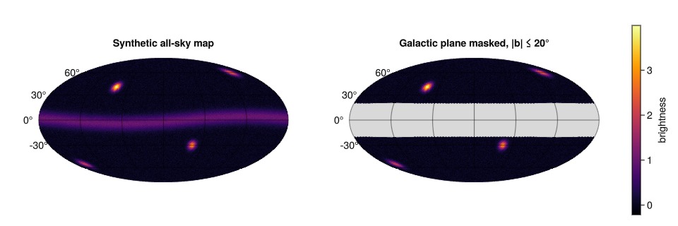

Cone search with a spherical cap

A spherical cone search selects cells whose polygons intersect a 5° cap. The cap is a SphericalCap, and Intersects wrapped in Cells makes it a normal dimension selector:

julia

lon0, lat0, _ = sources[1]
cone = GO.UnitSpherical.SphericalCap(to_sphere((lon0, lat0)), deg2rad(5))
incone = sky[DGG.Cells(DGG.Intersects(cone))]

┌ 114-element DimArray{Float64, 1} brightness ┐
├─────────────────────────────────────────────┴────────────────── dims ┐
  ↓ Cells CellLookup(HEALPixSystem, level=6, ncells=114, 16 windows)
└──────────────────────────────────────────────────────────────────────┘
 LevelIndex(6, 14863)  1.4371
 LevelIndex(6, 14872)  1.11776
 LevelIndex(6, 14873)  1.41949
 LevelIndex(6, 14874)  1.75995
 LevelIndex(6, 14875)  1.99689
 ⋮                     
 LevelIndex(6, 15045)  1.40289
 LevelIndex(6, 15046)  1.50027
 LevelIndex(6, 15048)  1.85521
 LevelIndex(6, 15049)  1.37133
 LevelIndex(6, 15050)  1.14576

Compare the cone mean with the all-sky mean:

julia

mean(incone), mean(sky)

(2.3107980288487835, 0.1447133253099803)

Within(cone) keeps only cells wholly inside the cap. The count difference identifies cells that cross the cap boundary:

julia

inside = sky[DGG.Cells(DGG.Within(cone))]
length(incone), length(inside)

(114, 68)

Running the same cone search on H3

The same selector works on another grid. Choose the H3 level closest in cell size to this HEALPix level, then run both boundary rules on the H3 field:

julia

h3 = DGG.levelgrid(DGG.H3System(), DGG.levelfor(DGG.H3System(), DGG.cellsize(grid)))
sky_h3 = synthetic_sky(h3)
incone_h3 = sky_h3[DGG.Cells(DGG.Intersects(cone))]
inside_h3 = sky_h3[DGG.Cells(DGG.Within(cone))]
length(incone_h3), length(inside_h3)

(99, 62)

The comparison figure uses one azimuthal-equidistant frame centred on the source. It distinguishes three sets:

dark purple: cells wholly inside the cone (Within);
light purple: cells crossing the rim, which Intersects adds;
gray: the surrounding sky.

julia

context = GO.UnitSpherical.SphericalCap(cone.point, deg2rad(11))

fig2 = Figure(size = (860, 430))
for (k, (g, A, met, within)) in enumerate([(grid, sky, incone, inside),
                                           (h3, sky_h3, incone_h3, inside_h3)])
    ax = GeoAxis(fig2[1, k]; dest = "+proj=aeqd +lon_0=$lon0 +lat_0=$lat0",
        limits = ((lon0 - 16, lon0 + 16), (lat0 - 12, lat0 + 12)),
        xgridvisible = false, ygridvisible = false,
        xticklabelsvisible = false, yticklabelsvisible = false,
        title = "$(nameof(typeof(DGG.system(g)))) level $(DGG.level(g)): " *
                "$(length(met)) meet the cone, $(length(within)) inside")
    dggpoly!(ax, A[DGG.Cells(DGG.Intersects(context))]; color = "#e9ecef",
        strokecolor = ("#212529", 0.35), strokewidth = 0.4)
    dggpoly!(ax, met; color = "#cbb3dd", strokecolor = "#f8f9fa", strokewidth = 0.6)
    dggpoly!(ax, within; color = "#9558b2", strokecolor = "#f8f9fa", strokewidth = 0.6)
    lines!(ax, rim; color = :black, linewidth = 2)
    scatter!(ax, [lon0], [lat0]; color = :white, strokecolor = :black,
        strokewidth = 1.2, marker = :star5, markersize = 16)
end
fig2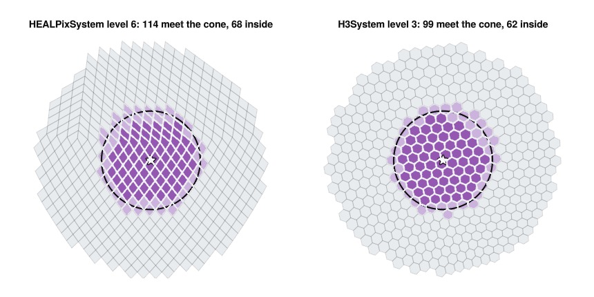

Doing it without the DimArray

A FITS reader may return a plain Vector. query returns the selected cell ids, and globalindex maps those ids to positions in the level grid, so the same cone statistic works without a DimArray:

julia

ids = DGG.query(grid, DGG.Intersects(cone))
idx = DGG.globalindex.(grid, ids)
mean(m.pixels[idx]) ≈ mean(incone)

true

This page was generated using Literate.jl.

The sky in HEALPix ​

Checking the pixel order against Healpix.jl ​

Building a synthetic sky as a DimArray over Cells ​

Masking the galactic plane ​

Cone search with a spherical cap ​

Running the same cone search on H3 ​

Doing it without the DimArray ​

The sky in HEALPix

Checking the pixel order against Healpix.jl

Building a synthetic sky as a DimArray over Cells

Masking the galactic plane

Cone search with a spherical cap

Running the same cone search on H3

Doing it without the DimArray