Stencil operations

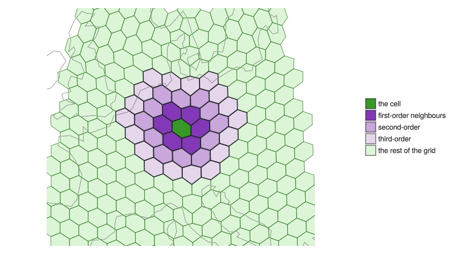
A stencil computes a new value from a cell and its neighbours. The figure shows successive rings of neighbours around one cell. Here we use stencils to smooth a field, detect its edges, request extra neighbour data, and compute a graph distance. Each example uses mapneighbors or the related adjacency table, so the same code can work with a different grid system.

Every field here is a DimArray with one Cells dimension. That dimension holds the lookup that connects array positions to cells and their neighbours.

import DiscreteGlobalGrids as DGG
import DimensionalData as DD
import GeometryOps as GO
import Extents
using DataStructures: PriorityQueue, enqueue!, dequeue_pair!
using Statistics, Random
using DiscreteGlobalGridsVisualization: dggpoly, dggpoly!
using GLMakie, GeoMakie
GLMakie.activate!(inline = true)

Building a field on the grid

A HEALPix grid at level 5, and its cells as a lookup that a dimension can hold:

grid = DGG.levelgrid(DGG.HEALPixSystem(), 5)

HierarchicalLevelGrid(HEALPixSystem, level=5, ncells=12288)

lookup = DGG.CellLookup(grid)

CellLookup(HEALPixSystem, level=5, ncells=12288, 1 windows)

We use cell centroids to define a reproducible test field. cell_centroid broadcasts over the lookup, and GeographicFromUnitSphere converts the returned unit-sphere points to longitude and latitude.

lonlat = GO.UnitSpherical.GeographicFromUnitSphere()
centroids = lonlat.(DGG.cell_centroid.(grid, lookup))
lon = DD.DimArray(first.(centroids), DGG.Cells(lookup); name = :lon)
lat = DD.DimArray(last.(centroids), DGG.Cells(lookup); name = :lat)

┌ 12288-element DimArray{Float64, 1} lat ┐
├────────────────────────────────────────┴──────────────────────── dims ┐
  ↓ Cells CellLookup(HEALPixSystem, level=5, ncells=12288, 1 windows)
└───────────────────────────────────────────────────────────────────────┘
 LevelIndex(5, 0)       1.19375
 LevelIndex(5, 1)       2.38802
 LevelIndex(5, 2)       2.38802
 LevelIndex(5, 3)       3.58332
 LevelIndex(5, 4)       3.58332
 ⋮                     
 LevelIndex(5, 12283)  -3.58332
 LevelIndex(5, 12284)  -3.58332
 LevelIndex(5, 12285)  -2.38802
 LevelIndex(5, 12286)  -2.38802
 LevelIndex(5, 12287)  -1.19375

The field combines a broad step, a longitude wave, and random noise. Any DimArray over the same Cells dimension can take its place, including a regridded raster or a column read from a store.

Random.seed!(42)
plateau = ifelse.(abs.(lat) .< 30, 8.0, 0.0)
wave = 3 .* sind.(2 .* lon) .* cosd.(lat)
field = DD.rebuild(plateau .+ wave .+ randn(length(lookup)); name = :value)

┌ 12288-element DimArray{Float64, 1} value ┐
├──────────────────────────────────────────┴────────────────────── dims ┐
  ↓ Cells CellLookup(HEALPixSystem, level=5, ncells=12288, 1 windows)
└───────────────────────────────────────────────────────────────────────┘
 LevelIndex(5, 0)      10.636
 LevelIndex(5, 1)      11.2455
 LevelIndex(5, 2)      10.6788
 LevelIndex(5, 3)      10.6829
 LevelIndex(5, 4)      11.796
 ⋮                     
 LevelIndex(5, 12283)   4.24406
 LevelIndex(5, 12284)   3.173
 LevelIndex(5, 12285)   5.99603
 LevelIndex(5, 12286)   5.45114
 LevelIndex(5, 12287)   5.87878

dggpoly draws the cells of such an array as one mesh, coloured by its values.

crange = extrema(field)

(-5.08079832071871, 13.904405750322002)

fig = Figure(size = (820, 460))
ax = GeoAxis(fig[1, 1]; dest = "+proj=moll", title = "the field",
    xgridcolor = (:black, 0.15), ygridcolor = (:black, 0.15))
dggpoly!(ax, field; color = parent(field), colormap = :viridis,
    colorrange = crange)
lines!(ax, GeoMakie.coastlines(); color = (:black, 0.45), linewidth = 0.5)
Colorbar(fig[1, 2]; colormap = :viridis, colorrange = crange, label = "value")
fig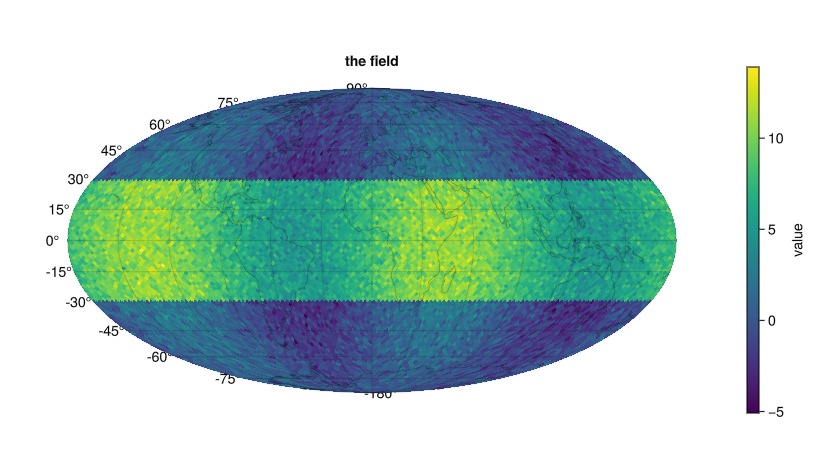

Smoothing with mapneighbors

mapneighbors applies a kernel once per cell and can thread those calls. Its default neighborhood is Disc(1). Use Disc(k) for all rings through k, or Ring(k) for cells at exactly k steps. With pass = Values(), the kernel receives f(cell, value, neighbours):

• value — the cell's own entry;

• neighbours — its neighbours' entries, counter-clockwise seen from outside the sphere, in the order neighbors fixes.

The neighbour order matters for oriented stencils such as gradients and upwind schemes. An average only needs the values. The result keeps the same Cells dimension.

smooth(A) = DGG.mapneighbors((c, x, nbs) -> (x + sum(nbs)) / (1 + length(nbs)),
    A; pass = DGG.Values())

smoothed = smooth(field)

┌ 12288-element DimArray{Float64, 1} value ┐
├──────────────────────────────────────────┴────────────────────── dims ┐
  ↓ Cells CellLookup(HEALPixSystem, level=5, ncells=12288, 1 windows)
└───────────────────────────────────────────────────────────────────────┘
 LevelIndex(5, 0)      10.8342
 LevelIndex(5, 1)      10.8183
 LevelIndex(5, 2)      10.3918
 LevelIndex(5, 3)      10.7198
 LevelIndex(5, 4)      10.8999
 ⋮                     
 LevelIndex(5, 12283)   4.49301
 LevelIndex(5, 12284)   4.85231
 LevelIndex(5, 12285)   5.29946
 LevelIndex(5, 12286)   4.57341
 LevelIndex(5, 12287)   4.99741

var(field), var(smoothed)

(19.91332414658947, 18.170830478579138)

Repeating the pass produces diffusion. Its result depends on multiple paths through intermediate cells, and each pass includes the center again. Two passes therefore do not equal one uniform average over a radius-two disk. Direct neighbors(grid, cell, 2) and ring(grid, cell, 2) queries are available, but the sweep API cannot yet apply either neighborhood across the whole field.

diffused = foldl((v, _) -> smooth(v), 1:10; init = field)
var(diffused)

16.082145715740513

neighborhood = Disc(3) widens one pass to every cell within three steps. The kernel is unchanged: nbs holds the three rings concatenated outward, in the order neighbors fixes, and the same average runs once over the whole disc. Ring(3) would hand it only the cells at exactly three steps.

wide = DGG.mapneighbors((c, x, nbs) -> (x + sum(nbs)) / (1 + length(nbs)),
    field; pass = DGG.Values(), neighborhood = DGG.Disc(3))
var(wide)

16.738979257789648

One pass at radius 3 and three one-ring passes are different computations. The disc pass weights every cell within three steps equally; the repeated passes compound, reaching a cell two steps away through every path of length two, so their weights fall off with distance. Choose the selector for a stencil of a given radius, and repetition for a diffusion process.

threepasses = foldl((v, _) -> smooth(v), 1:3; init = field)
maximum(abs, wide .- threepasses)

1.2536780599628785

Close up, over Europe and North Africa. Covering(box) selects every cell over a lon/lat box, and the result keeps its cell lookup, so dggpoly draws it as readily as the whole grid.

box = Extents.Extent(X = (-30.0, 50.0), Y = (18.0, 68.0))
patch = field[DGG.Cells(DGG.Covering(box))]

┌ 940-element DimArray{Float64, 1} value ┐
├────────────────────────────────────────┴─────────────────────── dims ┐
  ↓ Cells CellLookup(HEALPixSystem, level=5, ncells=940, 56 windows)
└──────────────────────────────────────────────────────────────────────┘
 LevelIndex(5, 61)    12.1705
 LevelIndex(5, 62)    10.4261
 LevelIndex(5, 63)     9.06981
 LevelIndex(5, 98)    11.2067
 LevelIndex(5, 99)    10.7484
 ⋮                    
 LevelIndex(5, 5115)   0.238414
 LevelIndex(5, 5116)   0.134818
 LevelIndex(5, 5117)   0.914966
 LevelIndex(5, 5118)  -0.935765
 LevelIndex(5, 5119)  -0.140864

zrange = extrema(patch)

(-4.323999745955703, 12.855563709321238)

fig = Figure(size = (900, 420))
for (k, (name, v)) in enumerate(("original" => field,
                                 "after 10 smoothing passes" => diffused))
    panel = GeoAxis(fig[1, k]; dest = "+proj=laea +lat_0=42 +lon_0=10",
        limits = ((-14.0, 34.0), (28.0, 58.0)), title = name,
        xgridvisible = false, ygridvisible = false,
        xticklabelsvisible = false, yticklabelsvisible = false)
    sub = v[DGG.Cells(DGG.Covering(box))]
    dggpoly!(panel, sub; color = parent(sub), colormap = :viridis,
        colorrange = zrange, strokecolor = (:white, 0.35), strokewidth = 0.3)
end
Colorbar(fig[1, 3]; colormap = :viridis, colorrange = zrange, label = "value")
fig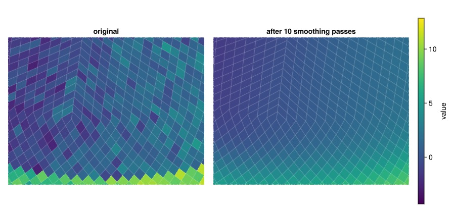

Detecting edges with the Laplacian

The discrete Laplacian compares a cell with the mean of its neighbours. Applying it after smoothing makes the step boundaries stand out as large second differences.

laplacian = DGG.mapneighbors((c, v, nbs) -> mean(nbs) - v, diffused;
    pass = DGG.Values())
extrema(laplacian)

(-0.1310172110789658, 0.12319662891949801)

The colour range uses the 95th percentile of the absolute Laplacian. This keeps ordinary texture visible while larger edge values use the clip colours.

q = quantile(abs.(laplacian), 0.95)

0.10011807504152823

fig = Figure(size = (820, 460))
ax = GeoAxis(fig[1, 1]; dest = "+proj=moll",
    title = "Laplacian of the smoothed field",
    xgridcolor = (:black, 0.15), ygridcolor = (:black, 0.15))
dggpoly!(ax, laplacian; color = parent(laplacian), colormap = :balance,
    colorrange = (-q, q), highclip = :darkred, lowclip = :darkblue)
Colorbar(fig[1, 2]; colormap = :balance, colorrange = (-q, q),
    highclip = :darkred, lowclip = :darkblue, label = "mean(neighbours) - centre")
fig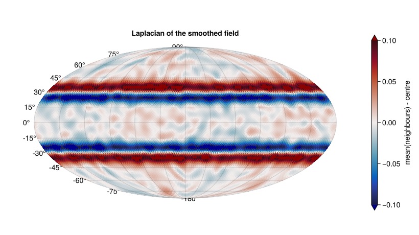

Reading more than one quantity per neighbour

needs declares the fields a kernel reads for each neighbour. This example requests values and centroids so it can measure a finite difference per unit great-circle distance.

function steepest((value, centre), (values, centres))
    isempty(values) && return 0.0
    maximum(eachindex(values)) do k
        arc = GO.UnitSpherical.spherical_distance(centres[k], centre)
        abs(values[k] - value) / (6371.0 * arc)   # 6371 km: the Earth's radius
    end
end

gradient = DGG.mapneighbors(steepest, field;
    needs = (DGG.Value(field), DGG.Centroid()))
extrema(gradient)   # units per kilometre

(0.0017602254057549336, 0.05793952309267872)

The callback is f(center, rings); both are tuples with one entry per need, in needs order:

	center	rings
need 1, Value(field)	the cell's value	every neighbour's value
need 2, Centroid()	the cell's centroid	every neighbour's centroid

Slot k of each ring is the same neighbour. Here is rings[1] for one cell, its eight neighbours' values:

valuerings = DGG.mapneighbors((centre, rings) -> first(rings), field;
    needs = (DGG.Value(field), DGG.Centroid()))
valuerings[1]

8-element SmallCollections.SmallVector{8, Float64}:
  9.984957950277078
 10.63819077941005
 11.23199904544338
 11.26084961958764
 11.245521424455651
 10.68288249042645
 10.678796237712467
 11.1484355816942

A kernel that wants one record per neighbour can combine the parallel rings with zip(rings...). Requesting neighbour fields documents the other available requests, including Cell() and Index(Local()).

Materialising the neighbour table with adjacency

adjacency materialises the neighbour lists once as a CSR table. Reuse it when many passes will traverse the same grid. Cells names the dimension to walk; mapneighbors inferred it in the earlier examples.

table = DGG.adjacency(field, DGG.Cells)

AdjacencyTable(halo = 0, ncells=12288, halocells=0, entries=98280)

Row i is neighbors(lookup, i) in the same order the sweep uses, so the table gives the same answer the sweep does:

[mean(vcat(field[i], field[table[i]])) for i in eachindex(field)] ≈ smoothed

true

Rows can have different lengths because the grid has cells with different degrees. HEALPix has fewer neighbours at cells around a base-tiling vertex:

sort(unique(length.(table))), count(==(7), length.(table))

([7, 8], 24)

Vertex() counts cells that share a corner, while Edge() keeps only cells that share a side. The next figure compares both neighbourhoods around the cell containing Zürich, selected with Contains:

p = only(DD.dims2indices(field, DGG.Cells(DD.Contains((8.5, 47.4)))))

695

disk = sort(vcat(p, DGG.neighbors(lookup, p, 3)))
shades = ["#dcf5d7", "#8338b8", "#389826"]

fig = Figure(size = (820, 420))
for (k, conn) in enumerate((DGG.Vertex(), DGG.Edge()))
    nbrs = DGG.neighbors(lookup, p; connectivity = conn)
    role = DD.DimArray(zeros(length(lookup)), DGG.Cells(lookup))
    parent(role)[nbrs] .= 1
    parent(role)[p] = 2
    panel = GeoAxis(fig[1, k]; dest = "+proj=laea +lat_0=47.4 +lon_0=8.5",
        title = "$(nameof(typeof(conn)))(): $(length(nbrs)) neighbours",
        xgridvisible = false, ygridvisible = false,
        xticklabelsvisible = false, yticklabelsvisible = false)
    around = role[disk]
    dggpoly!(panel, around; color = parent(around), colorrange = (0, 2),
        colormap = shades, strokecolor = "#2c7a1e", strokewidth = 1)
    hi = role[sort(vcat(p, nbrs))]
    dggpoly!(panel, hi; color = parent(hi), colorrange = (0, 2),
        colormap = shades, strokecolor = "#212529", strokewidth = 2.5)
end
fig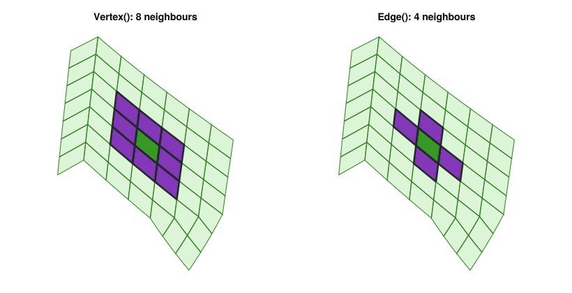

Running a stencil on a subset of the grid

A subset is itself a valid input. Its boundary cells see only neighbours that belong to the subset, so the same smooth call runs with a clipped stencil.

smoothed_patch = smooth(patch)
count(.!(parent(smoothed_patch) .≈ parent(smoothed[DGG.Cells(DGG.Covering(box))])))

151

The count identifies cells whose subset neighbourhood differs from the whole-grid result. Out of core shows how to load the margin a tile needs when boundary cells must agree with a full-grid pass.

Cost distance with Dijkstra

A cost field turns the cell graph into a travel network. The cost distance is the least accumulated cost from a seed, which Dijkstra's algorithm computes with a priority queue. neighbors(lookup, i) supplies the graph edges as local indices. This example measures cost per graph step; a travel cost per kilometre would also need the distance between cell centres.

function costdistance(cost, seed)
    lookup = DD.lookup(cost, DGG.Cells)
    source = only(DD.dims2indices(cost, DGG.Cells(DD.Contains(seed))))
    dist = fill(Inf, length(cost))
    dist[source] = 0.0
    queue = PriorityQueue{Int,Float64}()
    enqueue!(queue, source => 0.0)
    while !isempty(queue)
        i, d = dequeue_pair!(queue)
        d > dist[i] && continue          # a stale entry, already improved
        for j in DGG.neighbors(lookup, i)
            alt = d + (cost[i] + cost[j]) / 2
            if alt < dist[j]
                dist[j] = alt
                queue[j] = alt           # insert, or lower the key
            end
        end
    end
    return DD.rebuild(cost; data = dist, name = :costdistance)
end

costdistance (generic function with 1 method)

The example makes an equatorial wall impassable (Inf) except for a gap between 0° and 25° E. With Zürich as the seed, the resulting distance field shows how paths go around the wall or through the gap.

wall = @. (abs(lat) < 5) & !(0 <= lon <= 25)
cost = DD.rebuild(lat; data = ifelse.(wall, Inf, 1.0), name = :cost)
travel = costdistance(cost, (8.5, 47.4))
reach = maximum(filter(isfinite, parent(travel)))

93.0

The azimuthal-equidistant projection centres the map on the seed, making great-circle distance easy to compare visually. The map uses a 172° cap selected with Covering(cap).

centre = DGG.cell_centroid(grid, DGG.cellat(grid, 8.5, 47.4))
cap = GO.UnitSpherical.SphericalCap(centre, deg2rad(172))
near = travel[DGG.Cells(DGG.Covering(cap))]

┌ 12247-element DimArray{Float64, 1} costdistance ┐
├─────────────────────────────────────────────────┴──────────────── dims ┐
  ↓ Cells CellLookup(HEALPixSystem, level=5, ncells=12247, 12 windows)
└────────────────────────────────────────────────────────────────────────┘
 LevelIndex(5, 0)      Inf
 LevelIndex(5, 1)      Inf
 LevelIndex(5, 2)      Inf
 LevelIndex(5, 3)      Inf
 LevelIndex(5, 4)      Inf
 ⋮                     
 LevelIndex(5, 12283)  Inf
 LevelIndex(5, 12284)  Inf
 LevelIndex(5, 12285)  Inf
 LevelIndex(5, 12286)  Inf
 LevelIndex(5, 12287)  Inf

bands = cgrad(:viridis, 12; categorical = true)

fig = Figure(size = (960, 460))
ax = GeoAxis(fig[1, 1]; title = "cost of crossing a cell",
    dest = "+proj=aeqd +lat_0=47.4 +lon_0=8.5", xgridvisible = false,
    ygridvisible = false, xticklabelsvisible = false,
    yticklabelsvisible = false)
dggpoly!(ax, near; color = ifelse.(isinf.(parent(near)), 2.0, 1.0),
    colorrange = (1, 2), colormap = ["#eef3f7", "#b03030"])
lines!(ax, GeoMakie.coastlines(); color = (:black, 0.4), linewidth = 0.4)
scatter!(ax, [8.5], [47.4]; color = :dodgerblue, marker = :star5,
    markersize = 16, strokecolor = :black, strokewidth = 0.5)
ax = GeoAxis(fig[1, 2]; title = "cost distance from the seed",
    dest = "+proj=aeqd +lat_0=47.4 +lon_0=8.5", xgridvisible = false,
    ygridvisible = false, xticklabelsvisible = false,
    yticklabelsvisible = false)
dggpoly!(ax, near; color = parent(near), colormap = bands,
    colorrange = (0, reach), highclip = "#8c1b1b")
lines!(ax, GeoMakie.coastlines(); color = (:black, 0.4), linewidth = 0.4)
scatter!(ax, [8.5], [47.4]; color = :red, marker = :star5, markersize = 16,
    strokecolor = :black, strokewidth = 0.5)
Colorbar(fig[1, 3]; colormap = bands, colorrange = (0, reach),
    highclip = "#8c1b1b", label = "cost distance")
fig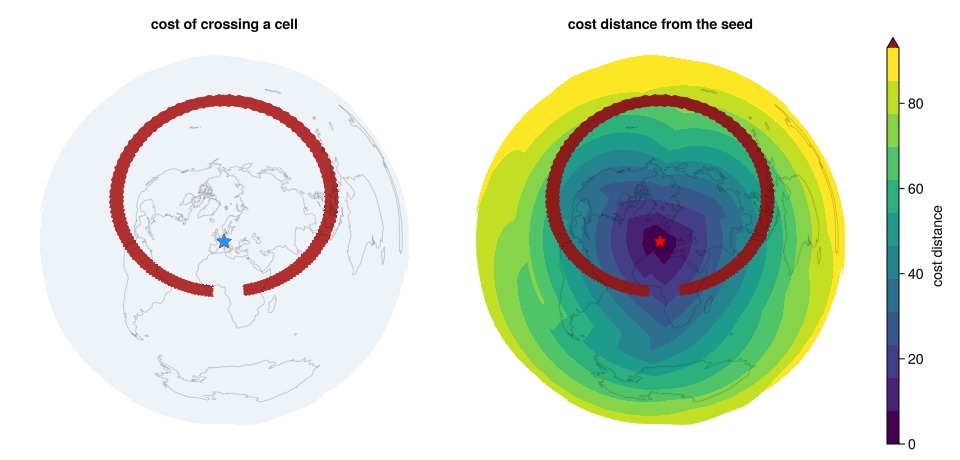

The bands bend around the wall and spread from the gap on its far side. The Inf wall is drawn in dark red above the distance scale.

Sweeping a plain vector of values

The same sweeps take the cells and the values as two arguments, for code that holds them apart:

cells = DGG.CellVector(grid)
values = parent(field)
DGG.mapneighbors((c, x, nbs) -> (x + sum(nbs)) / (1 + length(nbs)), cells,
    values) ≈ parent(smoothed)

true

Running the page on another grid system

levelgrid, mapneighbors, adjacency, and neighbors share the same interface across grid systems. Switching the constructor changes the cell topology while the stencil code stays the same. Choosing a grid compares those topology choices.

---

This page was generated using Literate.jl.