Multi-order coverage

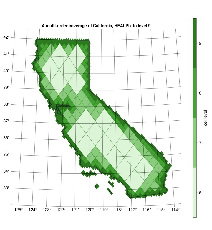
A multi-order coverage represents a region with cells at several levels. Coarse cells describe interior areas; finer cells follow the boundary. This gives a compact regional index while retaining a controllable finest resolution.

Each stored parent represents all of its descendants at the reference level. level_ranges exposes those leaves when the system has sorted subtrees. The descendants' union equals the parent's polygon only with congruent refinement, as in HEALPix, S2, and ISEA4R. IGeo7, H3, and A5 differ.

Mode	Meaning	Guarantee
level=l	Refine boundary crossings to a fixed finest level	Expansion includes all intersecting level-l cells; equality holds with congruent refinement
maxcells=n	Refine within a cell budget	A seed larger than n stays over budget; full coverage is guaranteed only with congruent refinement

On noncongruent systems, budget results can miss target polygons and intersecting reference-level cells. Displayed members and expanded leaves therefore answer different geometric questions.

Query California as a coverage in HEALPix

MultiOrderCoverage is a query target. Hand it a region and the finest level you will accept, and the query answers with the mixed-level set.

import DiscreteGlobalGrids as DGG
import NaturalEarth
import GeometryOps as GO, GeoInterface as GI
using DiscreteGlobalGridsVisualization: dggpoly, dggpoly!
using GLMakie, GeoMakie
GLMakie.activate!(inline = true)

fc = NaturalEarth.naturalearth("admin_1_states_provinces", 10)
california = fc.geometry[findfirst(==("California"), fc.name)]

2D MultiPolygonwith 8 sub-geometries

sys = DGG.HEALPixSystem()
moc = DGG.query(sys, DGG.MultiOrderCoverage(california); level = 9)

MultiOrderCellSet(HEALPixSystem, 729 cells, levels 6:9)

level = 9 sets the finest cell the query may emit. Inspect its typical width in metres with the package's √area convention:

DGG.cellsize(sys, 9)

12733.636337407695

Every entry carries the level at which it was emitted. Counting by level shows how the representation spends its cells:

levels = DGG.level.(moc)
[l => count(==(l), levels) for l in minimum(levels):maximum(levels)]

4-element Vector{Pair{Int64, Int64}}:
 6 => 19
 7 => 36
 8 => 85
 9 => 589

level_ranges reads the set as sorted, disjoint ranges of level-9 indices. A lookup can slice those ranges without materialising every represented id:

ranges = DGG.level_ranges(moc, 9)

155-element Vector{UnitRange{Int64}}:
 600062:600064
 601400:601400
 601404:601408
 601420:601424
 601426:601472
 601489:601504
 601522:601522
 601525:601528
 601533:601600
 601687:601687
 ⋮
 629361:629363
 629377:629407
 629409:629423
 629425:629427
 629441:629443
 629505:629507
 632145:632154
 632156:632159
 634881:634883

Their total length is the number of level-9 leaves represented by the set:

sum(length, ranges)

2721

Put an elevation raster onto the coverage

A coverage can be the destination of regrid. The source here is CRU CL 2.0, a 10-arcminute land climatology whose :elv layer holds mean elevation in metres.

ENV["RASTERDATASOURCES_PATH"] = mkpath(get(ENV, "RASTERDATASOURCES_PATH", joinpath(tempdir(), "rasterdatasources")))
using Rasters, RasterDataSources
import NCDatasets
import DimensionalData as DD
import Extents
using Statistics

world = Raster(RasterDataSources.getraster(CRUCL2); name = :elv, lazy = true)
elevation = read(world[X(-125.5 .. -113.5), Y(32.0 .. 42.5)])
elevation = DD.rebuild(elevation; metadata = DD.NoMetadata())

┌ 72×63 Raster{Union{Missing, Float32}, 2} elv ┐
├──────────────────────────────────────────────┴───────────────────────── dims ┐
  ↓ X Mapped{Float64} -125.41666666666666:0.16666666666666666:-113.58333333333333 ForwardOrdered Regular Points,
  → Y Mapped{Float64} 32.08333333333332:0.16666666666666666:42.41666666666666 ForwardOrdered Regular Points
├────────────────────────────────────────────────────────────────────── raster ┤
  missingval: missing
  extent: Extent(X = (-125.41666666666666, -113.58333333333333), Y = (32.08333333333332, 42.41666666666666))
  crs: EPSG:4326
  mappedcrs: EPSG:4326
└──────────────────────────────────────────────────────────────────────────────┘
    ↓ →     32.0833     32.25       32.4167    …    42.25        42.4167
 -125.417     missing     missing     missing         missing      missing
 -125.25      missing     missing     missing         missing      missing
 -125.083     missing     missing     missing         missing      missing
 -124.917     missing     missing     missing         missing      missing
    ⋮                                          ⋱               
 -114.083  142.0       281.0       300.0          1923.0       1352.0
 -113.917  228.0       357.0       330.0       …  1449.0       1325.0
 -113.75   292.0       383.0       274.0          1804.0       1362.0
 -113.583  261.0       311.0       248.0          1990.0       1558.0

The crop is a box and therefore includes a margin around California. surface! draws the source raster on the same GeoAxis used for cells; the z translation keeps the state outline visible above it:

albers = "+proj=aea +lat_1=34 +lat_2=40.5 +lat_0=0 +lon_0=-120 +datum=WGS84"

fig = Figure(size = (700, 760))
ax = GeoAxis(fig[1, 1]; dest = albers, limits = ((-125.5, -113.5), (32.0, 42.5)),
    title = "CRU CL 2.0 elevation, 10 arcmin")
plt = surface!(ax, replace_missing(elevation, NaN);
    colormap = :batlow, shading = NoShading)
translate!(plt, 0, 0, -100)
poly!(ax, california; color = :transparent,
    strokecolor = ("#212529", 0.9), strokewidth = 1.5)
Colorbar(fig[1, 2], plt; label = "elevation (m)")
fig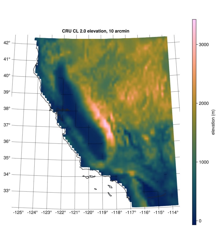

regrid takes the coverage as its destination:

A = DGG.regrid(elevation; to = moc)

┌ 2721-element Raster{Union{Missing, Float32}, 1} elv ┐
├─────────────────────────────────────────────────────┴──────────── dims ┐
  ↓ Cells CellLookup(HEALPixSystem, level=9, ncells=2721, 155 windows)
├──────────────────────────────────────────────────────────────── raster ┤
  missingval: missing
  extent: Extent(Cells = (LevelIndex(9, 600061), LevelIndex(9, 634882)),)
└────────────────────────────────────────────────────────────────────────┘
 LevelIndex(9, 600061)   15.8944
 LevelIndex(9, 600062)    7.00621
 LevelIndex(9, 600063)    9.52392
 LevelIndex(9, 601399)  730.773
 LevelIndex(9, 601403)  254.89
 ⋮                      
 LevelIndex(9, 632157)  662.382
 LevelIndex(9, 632158)  283.127
 LevelIndex(9, 634880)  804.604
 LevelIndex(9, 634881)  896.152
 LevelIndex(9, 634882)  772.071

The result is a Raster over one Cells dimension, with one value per represented level-9 leaf. Offshore cells remain missing because the source covers land:

count(ismissing, A)

69

DimensionalData's selectors read that axis. DD.Contains picks the cell holding a point — spelled through DD because this package exports DE9IM's Contains, a geometry predicate:

A[DGG.Cells(DD.Contains((-118.24, 34.05)))]  # Los Angeles

130.21985f0

Covering takes a region and answers with a smaller Raster whose axis is a cell axis again, so a statistic over a subregion is one more line:

sierra = A[DGG.Cells(DGG.Covering(Extents.Extent(X = (-119.5, -118.0), Y = (36.5, 38.0))))]

┌ 163-element Raster{Union{Missing, Float32}, 1} elv ┐
├────────────────────────────────────────────────────┴─────────── dims ┐
  ↓ Cells CellLookup(HEALPixSystem, level=9, ncells=163, 24 windows)
├────────────────────────────────────────────────────────────── raster ┤
  missingval: missing
  extent: Extent(Cells = (LevelIndex(9, 624085), LevelIndex(9, 627264)),)
└──────────────────────────────────────────────────────────────────────┘
 LevelIndex(9, 624085)   591.777
 LevelIndex(9, 624086)   210.637
 LevelIndex(9, 624087)   679.579
 LevelIndex(9, 624089)   105.507
 LevelIndex(9, 624090)    94.8654
 ⋮                      
 LevelIndex(9, 627226)  2732.83
 LevelIndex(9, 627227)  2886.38
 LevelIndex(9, 627228)  2635.01
 LevelIndex(9, 627248)  2696.51
 LevelIndex(9, 627264)  2163.96

mean(skipmissing(sierra))

2044.2742f0

replace_missing puts NaN in the missing cells, and dggpoly! leaves those cells undrawn:

A = replace_missing(A, NaN)

fig = Figure(size = (700, 760))
ax = GeoAxis(fig[1, 1]; dest = albers, limits = ((-125.5, -113.5), (32.0, 42.5)),
    title = "Elevation on the coverage, HEALPix to level 9")
plt = dggpoly!(ax, A; color = A, colormap = :batlow)
poly!(ax, california; color = :transparent,
    strokecolor = ("#212529", 0.9), strokewidth = 1.5)
Colorbar(fig[1, 2], plt; label = "elevation (m)")
fig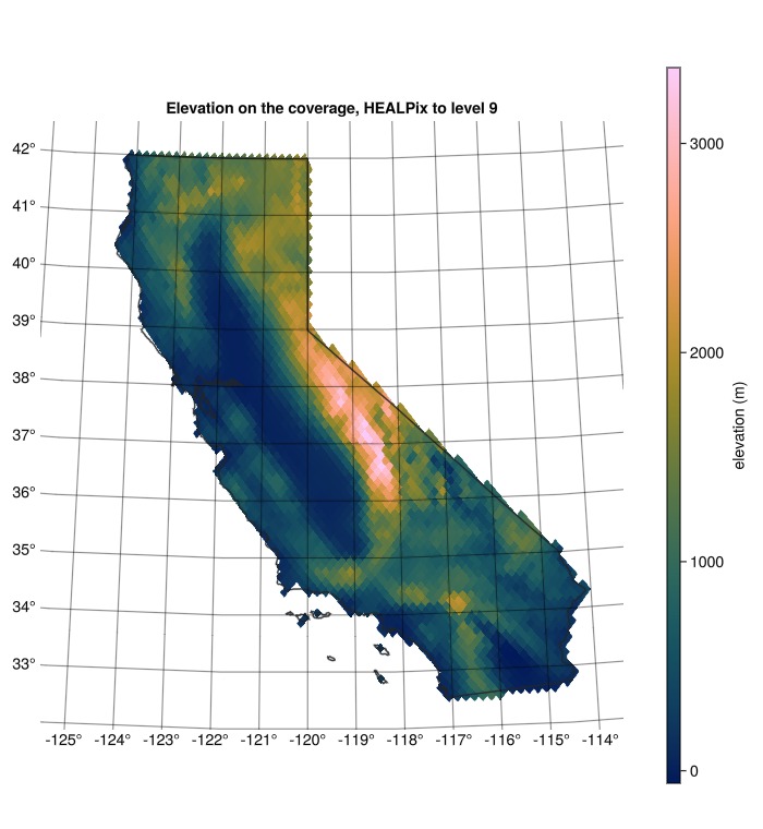

The map shows the regional relief while preserving the coverage's boundary rule: cells that meet California remain in the representation, so expanding the coverage produces a superset around the state outline.

Set a refinement budget with maxcells

maxcells chooses a space budget for the representation. The query refines the coarsest boundary cells first and stops when further refinement would exceed that budget. If the initial seed already exceeds maxcells, the result retains the seed and exceeds the budget. This HEALPix example has congruent refinement; the same coverage guarantee does not hold for IGeo7, H3, or A5.

1. Take the coarsest cell the outline crosses.

2. Replace it by the children that meet California.

3. Keep it whole when the replacement would exceed the budget.

Cells already proven inside the state stay as they are.

budgets = (10, 40, 100)
sets = [DGG.query(sys, DGG.MultiOrderCoverage(california); maxcells = n) for n in budgets]

3-element Vector{MultiOrderCellSet{HEALPixSystem, LevelIndex}}:
 MultiOrderCellSet(HEALPixSystem, 10 cells, levels 4:8)
 MultiOrderCellSet(HEALPixSystem, 40 cells, levels 5:9)
 MultiOrderCellSet(HEALPixSystem, 100 cells, levels 6:11)

Each result can span a different range of levels. The panels use one colour scale so the effect of the budget is easy to compare:

levelrange = extrema(DGG.level(c) for set in sets for c in set)

(4, 11)

budgettints = cgrad(["#dcf5d7", "#9fd894", "#5cb84c", "#389826", "#2c7a1e"],
    levelrange[2] - levelrange[1] + 1; categorical = true)

fig = Figure(size = (1000, 430))
for (k, (n, set)) in enumerate(zip(budgets, sets))
    local panel = GeoAxis(fig[1, k]; dest = albers,
        limits = ((-127.0, -112.0), (30.0, 44.0)), title = "maxcells = $n",
        xticklabelsvisible = false, yticklabelsvisible = false,
        xgridvisible = false, ygridvisible = false)
    dggpoly!(panel, set; color = DGG.level.(set), colormap = budgettints,
        colorrange = (levelrange[1] - 0.5, levelrange[2] + 0.5),
        strokecolor = "#2c7a1e", strokewidth = 0.5)
    poly!(panel, california; color = :transparent,
        strokecolor = ("#212529", 0.9), strokewidth = 1.0)
end
Colorbar(fig[1, 4]; colormap = budgettints,
    colorrange = (levelrange[1] - 0.5, levelrange[2] + 0.5),
    ticks = levelrange[1]:levelrange[2], label = "cell level")
fig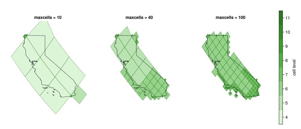

The same coverage on IGeo7

IGeo7 level 6 cells come nearest the 10-arcminute source in width:

igeo7 = DGG.IGeo7System()
DGG.cellsize(igeo7, 6)

20821.83616194328

moc7 = DGG.query(igeo7, DGG.MultiOrderCoverage(california); level = 6)

MultiOrderCellSet(IGeo7System, 414 cells, levels 4:6)

levels7 = DGG.level.(moc7)
lo7, hi7 = extrema(levels7)
tints7 = cgrad(["#dcf5d7", "#9fd894", "#5cb84c", "#389826", "#2c7a1e"],
    hi7 - lo7 + 1; categorical = true)

fig = Figure(size = (720, 780))
ax = GeoAxis(fig[1, 1]; dest = albers, limits = ((-125.5, -113.5), (32.0, 42.5)),
    title = "A multi-order coverage of California, IGeo7 to level 6")
plt = dggpoly!(ax, moc7; color = levels7, colormap = tints7,
    colorrange = (lo7 - 0.5, hi7 + 0.5),
    strokecolor = "#2c7a1e", strokewidth = 0.4)
poly!(ax, california; color = :transparent,
    strokecolor = ("#212529", 0.9), strokewidth = 1.6)
Colorbar(fig[1, 2], plt; ticks = lo7:hi7, label = "cell level")
fig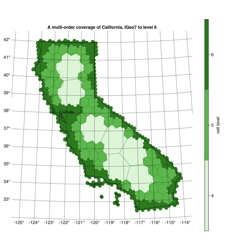

Mixed-level geometry follows the hierarchy of each system. HEALPix children tile their parent, while IGeo7's child footprints can overlap a coarser neighbour where the level changes. The leaf-level coverage guarantee remains the same: every finest cell that meets the region is represented by a member or one of its descendants. MultiOrderCoverage documents the system-specific coverage traits.

The raster regrids onto it by the same call:

A7 = replace_missing(DGG.regrid(elevation; to = moc7), NaN)

┌ 1056-element Raster{Float64, 1} elv ┐
├─────────────────────────────────────┴────────────────────────── dims ┐
  ↓ Cells CellLookup(IGeo7System, level=6, ncells=1056, 115 windows)
├────────────────────────────────────────────────────────────── raster ┤
  missingval: NaN
  extent: Extent(Cells = (Z7Cell("01462462"), Z7Cell("02156555")),)
└──────────────────────────────────────────────────────────────────────┘
 Z7Cell("01462462")   NaN
 Z7Cell("01462466")   NaN
 Z7Cell("01462640")  1169.58
 Z7Cell("01462644")   985.99
 Z7Cell("01462645")  1125.16
 ⋮                   
 Z7Cell("02156551")   338.559
 Z7Cell("02156552")   199.748
 Z7Cell("02156553")   370.442
 Z7Cell("02156554")   173.302
 Z7Cell("02156555")   266.446

fig = Figure(size = (700, 760))
ax = GeoAxis(fig[1, 1]; dest = albers, limits = ((-125.5, -113.5), (32.0, 42.5)),
    title = "Elevation on the coverage, IGeo7 to level 6")
plt = dggpoly!(ax, A7; color = A7, colormap = :batlow)
poly!(ax, california; color = :transparent,
    strokecolor = ("#212529", 0.9), strokewidth = 1.5)
Colorbar(fig[1, 2], plt; label = "elevation (m)")
fig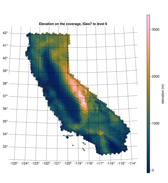

Work directly with cell collections

regrid and the selectors read the coverage through the calls below. Reach for them when you want the cell ids themselves.

CellLookup reads a set as a one-level cell axis. Its window count reports the contiguous runs used to represent the leaf ids:

lk = DGG.CellLookup(moc)

CellLookup(HEALPixSystem, level=9, ncells=2721, 155 windows)

expand flattens the set to one level as a CellVector, which is useful when an algorithm needs explicit cell ids:

flat = DGG.expand(moc, 9)

CellVector(HEALPixSystem, level=9, ncells=2721, 155 windows)

compact merges complete sibling groups into parents wherever membership permits. It uses membership alone and can therefore produce a shorter representation than the queried coverage:

DGG.compact(flat)

MultiOrderCellSet(HEALPixSystem, 339 cells, levels 5:9)

level_ranges needs contiguous subtrees (has_sorted_subtrees); expand works on every system.

A budgeted set records cells proven to lie inside the target. coarsest_contained returns the shallowest such cell, or nothing when the set contains no wholly contained cell:

DGG.coarsest_contained(sets[1])

Compare with the larger budget:

DGG.coarsest_contained(sets[2])

LevelIndex(6, 9399)

Cell areas over the coverage's leaves, in steradians. Equal-area systems make an unweighted mean over those leaves an areal mean:

g9 = DGG.levelgrid(sys, 9)
extrema(DGG.cell_area(g9, c) for c in flat)

(3.994741635118857e-6, 3.994741635118857e-6)

A budget set can back the same axis: CellLookup expands its mixed-level cells to the requested leaf level.

DGG.CellLookup(sets[2]; level = 9)

CellLookup(HEALPixSystem, level=9, ncells=3586, 23 windows)

Optional: reproduce the coverage walk

The earlier sections are the practical API. This optional section shows how a coverage query can be assembled from the hierarchy when you need a custom predicate or traversal. The walk is depth-first over the tree exposed by DGG.treeify; each node supplies an extent, a cell, its leaf status, and its children. At each node, the search:

1. drops the node when its cap misses the target;

2. drops the node when its cell polygon misses the target;

3. emits the cell when it is a leaf, or when its polygon lies inside the target;

4. visits the children when further refinement is needed.

import GeometryOps.SpatialTreeInterface as STI
import GeometryOps.UnitSpherical as US

The predicates run on the sphere, so the region moves to unit-sphere coordinates once. Float64 because RelateNG works in double precision and Natural Earth ships Float32:

tosphere = US.UnitSphereFromGeographic()
onsphere(geom) = GO.transform(p -> tosphere((Float64(GI.x(p)), Float64(GI.y(p)))), geom)

onsphere (generic function with 1 method)

A node's extent is a SphericalCap, so the target needs one too: centred on its centroid, with the radius reaching its farthest vertex.

function boundingcap(geom)
    centre = tosphere(GO.centroid(geom))
    radius = maximum(US.spherical_distance(centre, tosphere(p))
                     for p in GO.flatten(GI.PointTrait, geom))
    return US.SphericalCap(centre, radius)
end

boundingcap (generic function with 1 method)

cell_polygon returns a cell as a closed unit-sphere polygon for a cell id at any level, given that level's grid; levelgrid is a lightweight view of the system, so the walk asks for one at each cell it visits:

cellpolygon(sys, c) = DGG.cell_polygon(DGG.levelgrid(sys, DGG.level(c)), c)

cellpolygon (generic function with 1 method)

function coverage(sys, region, maxlevel)
    target = onsphere(region)
    cap = boundingcap(region)
    prepared = GO.prepare(GO.RelateNG(; manifold = GO.Spherical()), target)
    meets(poly) = GO.relate_predicate(prepared, GO.pred_intersects(), poly)
    inside(poly) = GO.relate_predicate(prepared, GO.pred_contains(), poly)
    out = DGG.cellindextype(sys)[]
    function visit(node)
        Extents.intersects(cap, STI.node_extent(node)) || return nothing
        c = DGG.node_cell(node)   # `nothing` at the synthetic root above the base cells
        if c !== nothing
            poly = cellpolygon(sys, c)
            meets(poly) || return nothing
            if STI.isleaf(node) || inside(poly)
                push!(out, c)
                return nothing
            end
        end
        for child in STI.getchild(node)
            visit(child)
        end
        return nothing
    end
    visit(DGG.treeify(DGG.levelgrid(sys, maxlevel)))
    return out
end

coverage (generic function with 1 method)

Compare it with query at level 7:

walked7 = coverage(sys, california, 7)
queried7 = DGG.query(sys, DGG.MultiOrderCoverage(california); level = 7)
length(walked7), length(queried7), Set(walked7) == Set(queried7)

(148, 148, true)

And at level 9, the coverage this page has been using:

walked9 = coverage(sys, california, 9)
length(walked9), length(moc), Set(walked9) == Set(moc)

(729, 729, true)

The sets agree. query accelerates this same traversal with subtree rejection from bounding caps and a cheaper acceptance test for cells whose centroids are inside the target.

---

This page was generated using Literate.jl.