Regridding: getting data onto a grid
Use regrid to bring a longitude/latitude raster onto a global grid. The result keeps its time dimension and works with the package's spatial selectors, neighbourhood operations and plotting tools.
Here we move twelve months of soil moisture onto HEALPix, choose how to handle missing ocean values, and map the result back to a raster. We use the default Conservative() method, which weights source values by their overlap with each destination cell. Moving between DGGS compares area averaging with point interpolation.
ENV["RASTERDATASOURCES_PATH"] = mkpath(get(ENV, "RASTERDATASOURCES_PATH", joinpath(tempdir(), "rasterdatasources")))

import DiscreteGlobalGrids as DGG
import DimensionalData as DD
using Rasters, RasterDataSources
import NCDatasets
import Dates
using Statistics
using GLMakie, GeoMakie
using DiscreteGlobalGridsVisualization: dggpoly, dggpoly!
GLMakie.activate!(inline = true)
The source: CPC soil moisture on a half-degree raster
The data is a monthly climatology from the NOAA Climate Prediction Center: one soil moisture value per half-degree lon/lat cell per month.
soil = Rasters.set(Raster(RasterDataSources.getraster(CPCSoil; period = "1981-2010");
    name = :soilw), Ti => 1:12)
soil = DD.rebuild(soil; metadata = DD.NoMetadata())
┌ 720×360×12 Raster{Union{Missing, Float32}, 3} soilw ┐
├─────────────────────────────────────────────────────┴────────── dims ┐
↓ X Mapped{Float64} 0.25:0.5:359.75 ForwardOrdered Regular Points,
→ Y Mapped{Float64} 89.75:-0.5:-89.75 ReverseOrdered Regular Points,
↗ Ti Sampled{Int64} 1:12 ForwardOrdered Regular Points
├────────────────────────────────────────────────────────────── raster ┤
missingval: missing
extent: Extent(X = (0.25, 359.75), Y = (-89.75, 89.75), Ti = (1, 12))
crs: EPSG:4326
mappedcrs: EPSG:4326
└──────────────────────────────────────────────────────────────────────┘
[:, :, 1]
↓ → 89.75 89.25 88.75 … -89.25 -89.75
0.25 missing missing missing 1.86265f-6 1.86265f-6
0.75 missing missing missing 1.86265f-6 1.86265f-6
1.25 missing missing missing 1.86265f-6 1.86265f-6
⋮ ⋱ ⋮
358.25 missing missing missing 1.86265f-6 1.86265f-6
358.75 missing missing missing 1.86265f-6 1.86265f-6
359.25 missing missing missing 1.86265f-6 1.86265f-6
359.75 missing missing missing … 1.86265f-6 1.86265f-6Every missing cell is ocean — the source measures land — and the ocean is most of the raster:
count(ismissing, soil) / length(soil)0.636917438271605The January map shows the source on its 0 … 360 longitude axis. regrid handles that longitude convention directly; the ocean remains missing.
fig, ax, plt = heatmap(soil[Ti = 1]; colormap = :viridis,
    axis = (; title = "January", xlabel = "longitude", ylabel = "latitude"))
Colorbar(fig[1, 2], plt; label = "soil moisture (mm)")
fig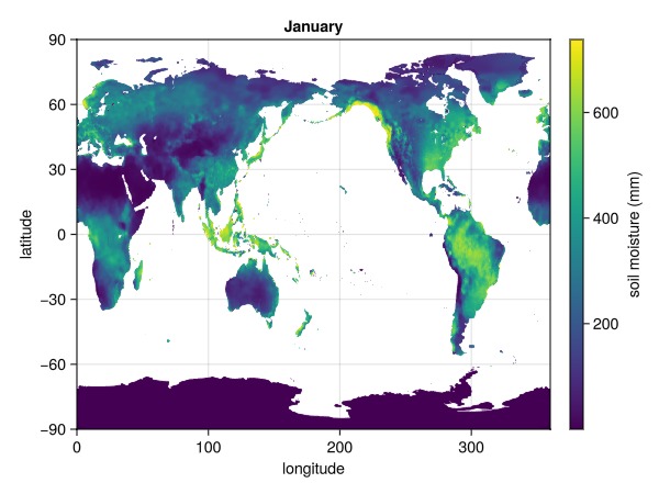
Regrid the raster onto HEALPix
HEALPix gives each cell the same area, which simplifies spatial averages. Choose a resolution close to the source with levelfor, then build that level with levelgrid. Choosing a grid explains cell sizes and coordinate conventions.
sys = DGG.HEALPixSystem()
grid = DGG.levelgrid(sys, DGG.levelfor(sys, soil))
HierarchicalLevelGrid(HEALPixSystem, level=7, ncells=196608)Metres across a source cell, and across a destination cell:
DGG.cellsize(soil), DGG.cellsize(grid)(46751.3894410621, 50934.54534963078)One call regrids all twelve months:
onhealpix = DGG.regrid(soil; to = grid)┌ 196608×12 Raster{Union{Missing, Float32}, 2} soilw ┐
├────────────────────────────────────────────────────┴───────────── dims ┐
↓ Cells CellLookup(HEALPixSystem, level=7, ncells=196608, 1 windows),
→ Ti Sampled{Int64} 1:12 ForwardOrdered Regular Points
├──────────────────────────────────────────────────────────────── raster ┤
missingval: missing
extent: Extent(Cells = (LevelIndex(7, 0), LevelIndex(7, 196607)), Ti = (1, 12))
└────────────────────────────────────────────────────────────────────────┘
↓ → 1 … 10 11 12
LevelIndex(7, 0) missing missing missing missing
LevelIndex(7, 1) missing missing missing missing
LevelIndex(7, 2) missing missing missing missing
LevelIndex(7, 3) missing missing missing missing
⋮ ⋱ ⋮
LevelIndex(7, 196604) missing … missing missing missing
LevelIndex(7, 196605) missing missing missing missing
LevelIndex(7, 196606) missing missing missing missing
LevelIndex(7, 196607) missing missing missing missingThe result is a Raster with dimensions Cells and Ti: one value per cell per month. You can still select January with [Ti = 1].
Draw the result on the sphere
replace_missing turns the ocean cells into NaN, and dggpoly! leaves a NaN cell unpainted:
january = Rasters.replace_missing(onhealpix[Ti = 1], NaN)

fig = Figure(size = (820, 400))
ax = GeoAxis(fig[1, 1]; dest = "+proj=moll", title = "January")
plt = dggpoly!(ax, january; color = january, colormap = :viridis)
Colorbar(fig[1, 2], plt; label = "soil moisture (mm)")
fig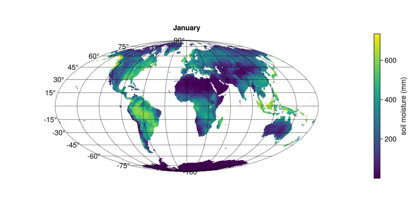
Read January's value at a few locations with DD.Contains((lon, lat)). The mid-Pacific query also checks how missing ocean data appears:
[place => onhealpix[DGG.Cells(DD.Contains((lon, lat))), Ti = DD.At(1)]
 for (place, lon, lat) in (("Amazon", -60.0, -5.0), ("Sahara", 15.0, 24.0),
                           ("Kansas", -100.0, 38.0), ("mid-Pacific", -150.0, 0.0))]
4-element Vector{Pair{String}}:
"Amazon" => 555.6809f0
"Sahara" => 2.3935847f0
"Kansas" => 252.00923f0
"mid-Pacific" => missingChoose what a coastal cell holds
A coastal cell can overlap both valid land values and missing ocean values. The default Weighted(0.5) averages the valid contribution and requires at least half of the total weight to be valid. A cell below that threshold gets a missing value.
Lowering the threshold keeps more coastal cells. Raising it asks for more complete coverage. Compare the number of valid January cells:
covered(t) = count(!ismissing, DGG.regrid(soil; to = grid,
    missingpolicy = DGG.Weighted(t))[:, 1])
[t => covered(t) for t in (0.01, 0.5, 1.0)]
3-element Vector{Pair{Float64, Int64}}:
0.01 => 67880
0.5 => 62315
1.0 => 56387The difference between these counts shows how much of the result depends on partial coverage. This raster uses missing for those cells. The regridding reference explains other missing value conventions and the Extensive() policy.
Reuse one plan across the twelve months
Reuse a regridding plan when several variables share the same source and destination grids. The plan computes the spatial weights once:
plan = DGG.plan_regrid(soil; to = grid)DirectPlan(Conservative, 196608 ← 259200 cells)Apply it to the full monthly cube:
monthly = DGG.regrid(soil, plan)┌ 196608×12 Raster{Union{Missing, Float32}, 2} soilw ┐
├────────────────────────────────────────────────────┴───────────── dims ┐
↓ Cells CellLookup(HEALPixSystem, level=7, ncells=196608, 1 windows),
→ Ti Sampled{Int64} 1:12 ForwardOrdered Regular Points
├──────────────────────────────────────────────────────────────── raster ┤
missingval: missing
extent: Extent(Cells = (LevelIndex(7, 0), LevelIndex(7, 196607)), Ti = (1, 12))
└────────────────────────────────────────────────────────────────────────┘
↓ → 1 … 10 11 12
LevelIndex(7, 0) missing missing missing missing
LevelIndex(7, 1) missing missing missing missing
LevelIndex(7, 2) missing missing missing missing
LevelIndex(7, 3) missing missing missing missing
⋮ ⋱ ⋮
LevelIndex(7, 196604) missing … missing missing missing
LevelIndex(7, 196605) missing missing missing missing
LevelIndex(7, 196606) missing missing missing missing
LevelIndex(7, 196607) missing missing missing missingUse regrid! to reuse an output array as well:
buffer = similar(monthly)
DGG.regrid!(buffer, soil, plan)
isequal(buffer, monthly)trueAnimate the seasonal cycle
A shared colour scale makes the months comparable. Animate the values on the same grid to see the seasonal cycle:
seasonal = Rasters.replace_missing(monthly, NaN)
crange = extrema(filter(!isnan, seasonal))
colors = Observable(seasonal[Ti = 1])
title = Observable(Dates.monthname(1))

fig = Figure(size = (820, 400))
ax = GeoAxis(fig[1, 1]; dest = "+proj=moll", title)
plt = dggpoly!(ax, seasonal[Ti = 1]; color = colors,
    colormap = :viridis, colorrange = crange)
Colorbar(fig[1, 2], plt; label = "soil moisture (mm)")

record(fig, "seasonal_soilw.mp4", 1:12; framerate = 2) do m
    colors[] = seasonal[Ti = m]
    title[] = Dates.monthname(m)
end
Regrid back onto a lon/lat raster
Use an existing raster as the destination template when a downstream tool expects longitude and latitude axes. Pass the source DGGS grid as from:
back = DGG.regrid(monthly; to = soil, from = grid)┌ 720×360×12 Raster{Union{Missing, Float32}, 3} soilw ┐
├─────────────────────────────────────────────────────┴────────────────── dims ┐
↓ X Sampled{Float64} 0.25:0.5:359.75 ForwardOrdered Explicit Intervals{Center},
→ Y Sampled{Float64} 89.75:-0.5:-89.75 ReverseOrdered Explicit Intervals{Center},
↗ Ti Sampled{Int64} 1:12 ForwardOrdered Regular Points
├────────────────────────────────────────────────────────────────────── raster ┤
missingval: missing
extent: Extent(X = (0.0, 360.0), Y = (-89.5, 89.5), Ti = (1, 12))
└──────────────────────────────────────────────────────────────────────────────┘
[:, :, 1]
↓ → 89.75 89.25 88.75 … -89.25 -89.75
0.25 missing missing missing 1.86265f-6 1.86265f-6
0.75 missing missing missing 1.86265f-6 1.86265f-6
1.25 missing missing missing 1.86265f-6 1.86265f-6
⋮ ⋱ ⋮
358.25 missing missing missing 1.86265f-6 1.86265f-6
358.75 missing missing missing 1.86265f-6 1.86265f-6
359.25 missing missing missing 1.86265f-6 1.86265f-6
359.75 missing missing missing … 1.86265f-6 1.86265f-6Compare the original and returned values where both are valid. These plain means are a useful check of the change in the field; they do not test area conservation, because longitude/latitude pixels have unequal areas. The round trip also retains the smoothing introduced by regridding.
both = .!ismissing.(soil) .&& .!ismissing.(back)
mean(soil[both]), mean(back[both])
(176.27245f0, 176.2389f0)You can also choose new destination coordinates. A -180 … 180 longitude axis fits the following world map:
shown = DGG.regrid(monthly[Ti = 1]; from = grid,
    to = Rasters.set(soil, X => -179.75:0.5:179.75))

fig = Figure(size = (820, 400))
ax = GeoAxis(fig[1, 1]; dest = "+proj=moll", title = "January, regridded twice")
plt = surface!(ax, Rasters.replace_missing(shown, NaN);
    colormap = :viridis, colorrange = crange, shading = NoShading)
Colorbar(fig[1, 2], plt; label = "soil moisture (mm)")
fig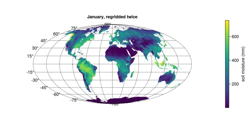
Regrid onto any other system
Choose another system and match its cell size to the same source:
igeo7 = DGG.IGeo7System()
DGG.regrid(soil; to = DGG.levelgrid(igeo7, DGG.levelfor(igeo7, soil)))
┌ 168072×12 Raster{Union{Missing, Float32}, 2} soilw ┐
├────────────────────────────────────────────────────┴─────────── dims ┐
↓ Cells CellLookup(IGeo7System, level=5, ncells=168072, 1 windows),
→ Ti Sampled{Int64} 1:12 ForwardOrdered Regular Points
├────────────────────────────────────────────────────────────── raster ┤
missingval: missing
extent: Extent(Cells = (Z7Cell("0000000"), Z7Cell("1166666")), Ti = (1, 12))
└──────────────────────────────────────────────────────────────────────┘
↓ → 1 … 10 11 12
Z7Cell("0000000") 353.251 295.696 320.829 338.593
Z7Cell("0000001") 383.954 322.687 347.234 366.558
Z7Cell("0000003") 400.948 334.315 359.172 380.128
Z7Cell("0000004") missing missing missing missing
⋮ ⋱ ⋮
Z7Cell("1166663") missing missing missing missing
Z7Cell("1166664") missing … missing missing missing
Z7Cell("1166665") missing missing missing missing
Z7Cell("1166666") missing missing missing missingThe result supports the same operations whichever system you choose. Try Zonal statistics to summarize it by region, or Stencil operations to compute from neighbouring cells.
For a different interpretation of the source values, see Choosing a regridding method.
This page was generated using Literate.jl.