Hydrology: a DEM on an IGEO7 grid
This tutorial takes a regional Copernicus DEM through IGEO7 regridding, D8 and D∞ flow routing, and a custom downhill-neighbour kernel with mapneighbors.
ENV["RASTERDATASOURCES_PATH"] = mkpath(get(ENV, "RASTERDATASOURCES_PATH", joinpath(tempdir(), "rasterdatasources")))

import DiscreteGlobalGrids as DGG
import Geomorphometry as GM
import GeoInterface as GI
using Rasters, RasterDataSources
import ArchGDAL
import Extents
using Statistics
using GLMakie, GeoMakie
using DiscreteGlobalGridsVisualization: dggsurface, dggsurface!, dggpoly, dggpoly!
GLMakie.activate!(inline = true)
Regrid a Copernicus DEM tile onto IGEO7 hexagons
One 1°×1° tile of the Copernicus DEM at 30 m over the Alps, fetched from its AWS Open Data bucket by RasterDataSources:
centre = GI.extent((10.5, 46.5))
path = only(skipmissing(RasterDataSources.getraster(CopernicusDEM; extent = centre)))
Sys.isapple() && Rasters.checkmem!(false) # needed for Apple systems
dem = Raster(path; lazy = false)
┌ 3600×3600 Raster{Float32, 2} ┐
├──────────────────────────────┴───────────────────────────────────────── dims ┐
↓ X Projected{Float64} 9.99986111111111:0.0002777777777777778:10.999583333333334 ForwardOrdered Regular Points,
→ Y Projected{Float64} 47.00013888888889:-0.0002777777777777778:46.000416666666666 ReverseOrdered Regular Points
├──────────────────────────────────────────────────────────────────── metadata ┤
Metadata{Rasters.GDALsource} of Dict{String, Any} with 1 entry:
"filepath" => "/tmp/rasterdatasources/CopernicusDEM/30m/Copernicus_DSM_COG_10…
├────────────────────────────────────────────────────────────────────── raster ┤
extent: Extent(X = (9.99986111111111, 10.999583333333334), Y = (46.000416666666666, 47.00013888888889))
crs: GEOGCS["WGS 84",DATUM["WGS_1984",SPHEROID["WGS 84",6378137,298.25722...
└──────────────────────────────────────────────────────────────────────────────┘
↓ → 47.0001 46.9999 46.9996 … 46.001 46.0007 46.0004
9.99986 1112.41 1112.34 1136.75 1769.15 1762.42 1753.84
10.0001 1105.91 1104.24 1129.33 1760.54 1758.42 1754.8
⋮ ⋱ ⋮
10.9993 1781.02 1783.85 1792.95 872.688 887.363 899.754
10.9996 1764.54 1765.67 1767.66 … 859.839 879.507 899.127These three calls choose a compatible resolution, select the cells touched by the tile, and transfer the DEM values onto that irregular cell set:
sys = DGG.IGeo7System()
leaf_level = DGG.levelfor(sys, dem)
region = DGG.query(sys, DGG.MultiOrderCoverage(Rasters.extent(dem)); level = leaf_level)
elevation = DGG.regrid(dem; to = region)
┌ 16172725-element Raster{Float32, 1} ┐
├─────────────────────────────────────┴────────────────────────────────── dims ┐
↓ Cells CellLookup(IGeo7System, level=13, ncells=16172725, 9887 windows)
├──────────────────────────────────────────────────────────────────── metadata ┤
Metadata{Rasters.GDALsource} of Dict{String, Any} with 1 entry:
"filepath" => "/tmp/rasterdatasources/CopernicusDEM/30m/Copernicus_DSM_COG_10…
├────────────────────────────────────────────────────────────────────── raster ┤
missingval: NaN32
extent: Extent(Cells = (Z7Cell("000622212313132"), Z7Cell("006115665666666")),)
└──────────────────────────────────────────────────────────────────────────────┘
Z7Cell("000622212313132") 2408.92
Z7Cell("000622212313133") 2418.06
Z7Cell("000622212313200") 2392.92
⋮
Z7Cell("006115665666664") 664.456
Z7Cell("006115665666665") 669.418
Z7Cell("006115665666666") 665.512regrid returns a Raster over a Cells axis. Copernicus DEM declares no source missing value, so cells outside the tile use the output convention NaN; pass missingval to choose a different fill value.
The level levelfor chose, and what its cells measure across:
leaf_level, DGG.cellsize(sys, leaf_level)(13, 22.944350401950622)The two panels show the source pixels and the regridded cells over the same terrain:
tile = Rasters.extent(dem)
lims = (tile.X, tile.Y)
shape = AxisAspect(cosd(46.5))            # a degree of longitude is cos(lat) as wide as a degree of latitude
crange = extrema(dem)

fig = Figure(size = (900, 470))
ax1 = Axis(fig[1, 1]; aspect = shape, limits = lims,
    xlabel = "longitude", ylabel = "latitude",
    title = "Copernicus DEM, $(size(dem, 1))×$(size(dem, 2)) pixels")
heatmap!(ax1, dem; colormap = :terrain, colorrange = crange)
ax2 = Axis(fig[1, 2]; aspect = shape, limits = lims,
    xlabel = "longitude", yticklabelsvisible = false,
    title = "IGEO7 level $leaf_level, $(round(length(elevation) / 1e6; digits = 1)) M cells")
p = dggsurface!(ax2, elevation; color = elevation,
    colormap = :terrain, colorrange = crange)
Colorbar(fig[1, 3], p; label = "elevation (m)")
fig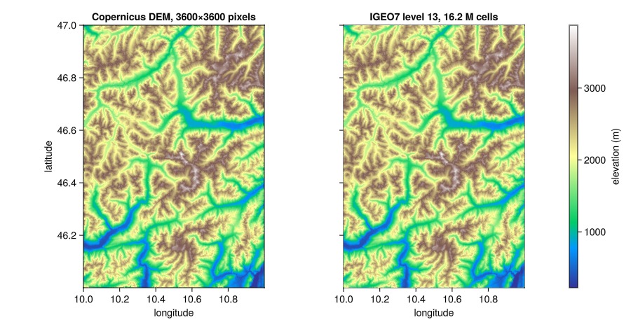
Represent a large region as a multi-order coverage
region is the coarsest hierarchical set of cells that covers the tile. It keeps large cells in the interior and refines cells near the boundary, where a large cell would extend beyond the tile. Its cell lookup expands that compact representation to the leaf cells:
length(region), length(DGG.CellLookup(region))(44197, 16172725)Colouring by level makes the compact hierarchy visible.
levels = DGG.level.(collect(region))

fig = Figure(size = (620, 540))
ax = Axis(fig[1, 1]; aspect = shape, limits = lims,
    xlabel = "longitude", ylabel = "latitude",
    title = "$(length(region)) coverage cells over $(length(DGG.CellLookup(region))) leaves")
heatmap!(ax, dem; colormap = :grays)
p = dggpoly!(ax, region; color = levels, alpha = 0.75,
    colormap = cgrad(:managua, length(unique(levels)); categorical = true),
    colorrange = (minimum(levels) - 0.5, maximum(levels) + 0.5),
    strokewidth = 0.15, strokecolor = (:black, 0.35))
Colorbar(fig[1, 2], p; label = "cell level", ticks = minimum(levels):maximum(levels))
fig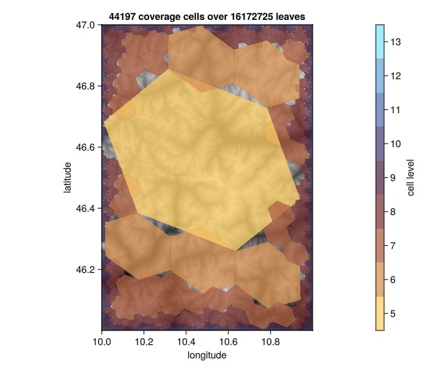
A coverage contains the extent, so boundary cells can extend beyond the tile. Those leaves have no source pixels and hold NaN:
count(isnan, elevation)14223The explicit limits keep the plot focused on the source tile.
Accumulate flow with D8
Geomorphometry's verbs take this raster as it is: they read neighbours and cell geometry off its Cells axis. One cell's area, in square metres:
area_per_cell = GM.cellarea(elevation, first(eachindex(elevation)))526.4432153672174flowaccumulation returns upstream area in square metres together with the directions used to route it. The default D8 method sends all of a cell's outflow to one neighbour:
accumulation, directions = GM.flowaccumulation(elevation)(Float32[526.44324, 526.44324, 12634.64, 12634.64, 11581.753, 12108.196, 13161.083, 13161.083, 12108.196, 11581.753 … 526.44324, 526.44324, 1052.8865, 526.44324, 526.44324, 526.44324, 526.44324, 1579.3297, 526.44324, 526.44324], Geomorphometry.FlowDirection{Geomorphometry.LDD, UInt8}[·, ·, ↘, ↘, ↘, ↘, ·, ·, ·, ↘ … ↑, ↖, ↖, ↘, ↖, ↑, ↖, ↘, ↗, ↘])Dividing by a representative cell area expresses accumulation in cell-area units. IGEO7 is approximately equal-area, so this is an approximate upstream cell count rather than an exact count:
log_cells = log10.(accumulation ./ area_per_cell)┌ 16172725-element Raster{Float64, 1} ┐
├─────────────────────────────────────┴────────────────────────────────── dims ┐
↓ Cells CellLookup(IGeo7System, level=13, ncells=16172725, 9887 windows)
├──────────────────────────────────────────────────────────────────── metadata ┤
Metadata{Rasters.GDALsource} of Dict{String, Any} with 1 entry:
"filepath" => "/tmp/rasterdatasources/CopernicusDEM/30m/Copernicus_DSM_COG_10…
├────────────────────────────────────────────────────────────────────── raster ┤
extent: Extent(Cells = (Z7Cell("000622212313132"), Z7Cell("006115665666666")),)
└──────────────────────────────────────────────────────────────────────────────┘
Z7Cell("000622212313132") 1.80975e-8
Z7Cell("000622212313133") 1.80975e-8
Z7Cell("000622212313200") 1.38021
⋮
Z7Cell("006115665666664") 0.477121
Z7Cell("006115665666665") 1.80975e-8
Z7Cell("006115665666666") 1.80975e-8Index a smaller extent to inspect the drainage pattern:
window = Extents.Extent(X = (10.30, 10.45), Y = (46.55, 46.68))
here = log_cells[DGG.Cells(DGG.Covering(window))]

fig = Figure(size = (640, 560))
ax = Axis(fig[1, 1]; aspect = shape, limits = (window.X, window.Y),
    xlabel = "longitude", ylabel = "latitude",
    title = "D8 flow accumulation, $(length(here)) cells")
p = dggsurface!(ax, here; color = here,
    colormap = :devon, colorrange = (1, 3.5), highclip = :white)
Colorbar(fig[1, 2], p; label = "log₁₀ cells upstream")
fig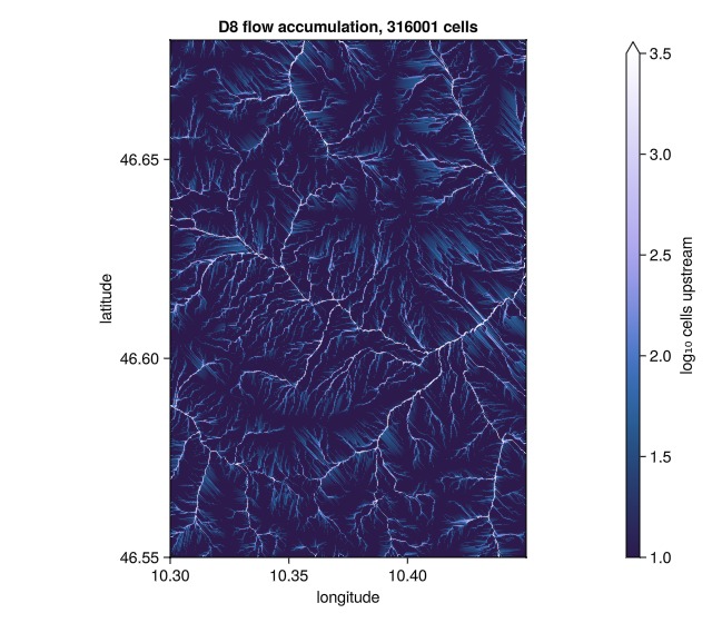
Split the flow between neighbours with D∞
D∞ (Tarboton 1997) splits each cell's outflow between the two neighbours that bracket its downslope direction, so hillslope flow fans out where D8 threads it through single cells. On a hexagon those two neighbours are ring slots, two of the six around each cell.
The example uses a padded box to reduce edge effects for the selected window. Padding helps capture upstream paths, but it cannot guarantee that every catchment is complete unless the box reaches each true divide:
padded = Extents.Extent(X = (10.20, 10.55), Y = (46.45, 46.78))
around = elevation[DGG.Cells(DGG.Covering(padded))]
accumulation_dinf, _ = GM.flowaccumulation(around; method = GM.DInf())
here_dinf = log10.(accumulation_dinf ./ area_per_cell)[DGG.Cells(DGG.Covering(window))]

fig = Figure(size = (640, 560))
ax = Axis(fig[1, 1]; aspect = shape, limits = (window.X, window.Y),
    xlabel = "longitude", ylabel = "latitude",
    title = "D∞ flow accumulation, $(length(here_dinf)) cells")
p = dggsurface!(ax, here_dinf; color = here_dinf,
    colormap = :devon, colorrange = (1, 3.5), highclip = :white)
Colorbar(fig[1, 2], p; label = "log₁₀ cells upstream")
fig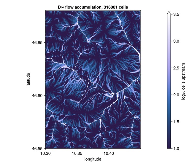
Find each cell's downhill neighbour by hand
This kernel demonstrates custom neighbourhood logic: each cell drains to the neighbour with the greatest elevation drop. mapneighbors supplies the elevation and local index for every ring neighbour:
function downhill((z, _), (zs, ids))
    isnan(z) && return (0, NaN32)
    dest, fall = 0, 0.0f0
    for k in eachindex(zs)
        isnan(zs[k]) && continue
        z - zs[k] > fall && ((dest, fall) = (ids[k], z - zs[k]))
    end
    return (dest, dest == 0 ? NaN32 : fall)
end

flow, drop = DGG.mapneighbors(downhill, elevation;
    needs = (DGG.Value(vec(elevation)), DGG.Index(DGG.Local())))
flow
┌ 16172725-element Raster{Int64, 1} ┐
├───────────────────────────────────┴──────────────────────────────────── dims ┐
↓ Cells CellLookup(IGeo7System, level=13, ncells=16172725, 9887 windows)
├──────────────────────────────────────────────────────────────────── metadata ┤
Metadata{Rasters.GDALsource} of Dict{String, Any} with 1 entry:
"filepath" => "/tmp/rasterdatasources/CopernicusDEM/30m/Copernicus_DSM_COG_10…
├────────────────────────────────────────────────────────────────────── raster ┤
extent: Extent(Cells = (Z7Cell("000622212313132"), Z7Cell("006115665666666")),)
└──────────────────────────────────────────────────────────────────────────────┘
Z7Cell("000622212313132") 70
Z7Cell("000622212313133") 1
Z7Cell("000622212313200") 7
⋮
Z7Cell("006115665666664") 16047930
Z7Cell("006115665666665") 16172723
Z7Cell("006115665666666") 16048041flow stores the selected downstream index and drop stores its elevation fall, one raster per returned component. The kernel leaves pits and cells outside the source coverage without a destination:
count(==(0), flow)95694The drop raster highlights steep local steps and leaves gentle valley floors dark. Because the kernel compares elevation differences only, it does not normalize the drop by neighbour distance or compute slope.
fig = Figure(size = (620, 540))
ax = Axis(fig[1, 1]; aspect = shape, limits = lims,
    xlabel = "longitude", ylabel = "latitude", title = "drop to the downhill neighbour")
p = dggsurface!(ax, drop; color = drop,
    colormap = :magma, colorrange = (0, 30), highclip = :white)
Colorbar(fig[1, 2], p; label = "metres")
fig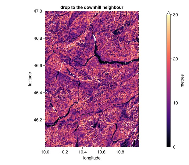
Compare the two sets of directions
directions from the D8 run holds one downstream neighbour per cell in Geomorphometry's local-drain-direction (LDD) code. Encoding flow the same way makes the two comparable:
cells = collect(lookup(elevation, DGG.Cells))
sends = vec(flow)
downstream(i) = sends[i] == 0 ? cells[i] : cells[sends[i]]
mine = [GM.FlowDirection{GM.LDD}(downstream(i) - cells[i]) for i in eachindex(cells)]

mean(mine .== directions)0.9876241635222265Differences occur where the one-ring rule stops at a pit. The library's D8 fills depressions and routes water over their rims. Where the custom kernel finds a lower neighbour, compare the resulting directions directly:
routed = findall(!=(0), sends)
mean(mine[routed] .== vec(directions)[routed])0.9932723274589692Which systems each method runs on
MultiOrderCoverage, regrid, and mapneighbors share the DGGS interface; their setup can be reused with another system. Among the Geomorphometry methods shown here, D8 is portable across systems, while the advanced methods require IGEO7 support for relative-cell arithmetic:
| verb | systems |
|---|---|
flowaccumulation with D8(), the default | any |
flowaccumulation with DInf() or FD8(), and height_above_nearest_drainage | IGEO7 — these need relative-cell arithmetic, which the IGEO7 backend provides |
This page was generated using Literate.jl.