Zonal statistics

A zonal statistic reduces the cells in each region to one value. This example estimates each country's mean July temperature from a HEALPix grid.

import DiscreteGlobalGrids as DGG
import DimensionalData as DD
import NaturalEarth
import NCDatasets  # the netCDF backend Rasters reads CRU through
using Rasters, RasterDataSources
using Statistics
using DiscreteGlobalGridsVisualization: dggpoly, dggpoly!
using GLMakie, GeoMakie
GLMakie.activate!(inline = true)

Load the July temperature raster

CRU CL 2.0 is a station climatology of 1961–1990 over land, at 10 arcmin. Its :tmp variable holds mean temperature in °C with one layer per month, and July is layer 7.

tavg = read(Raster(RasterDataSources.getraster(CRUCL2); name = :tmp, lazy = true)[Ti = 7])

┌ 2160×1080 Raster{Union{Missing, Float32}, 2} tmp ┐
├──────────────────────────────────────────────────┴───────────────────── dims ┐
  ↓ X Mapped{Float64} -179.91666666666666:0.16666666666666666:179.91666666666666 ForwardOrdered Regular Points,
  → Y Mapped{Float64} -89.91666666666667:0.16666666666666666:89.91666666666666 ForwardOrdered Regular Points
├──────────────────────────────────────────────────────────────────── metadata ┤
  Metadata{Rasters.NCDsource} of Dict{String, Any} with 3 entries:
  "_FillValue" => NaN
  "units"      => "C"
  "long_name"  => "mean temperature"
├────────────────────────────────────────────────────────────────────── raster ┤
  missingval: missing
  extent: Extent(X = (-179.91666666666666, 179.91666666666666), Y = (-89.91666666666667, 89.91666666666666))
  crs: EPSG:4326
  mappedcrs: EPSG:4326
└──────────────────────────────────────────────────────────────────────────────┘
    ↓ →    -89.9167    -89.75      …  89.5833    89.75      89.9167
 -179.917     missing     missing       missing    missing    missing
    ⋮                              ⋱                         ⋮
  179.917     missing     missing  …    missing    missing    missing

Ocean cells hold missing, and the source record has limited Antarctic coverage.

fig, ax, plt = heatmap(tavg; colormap = :thermal,
    axis = (; aspect = DataAspect(), title = "CRU CL 2.0 mean July temperature"))
Colorbar(fig[1, 2], plt; label = "°C")
fig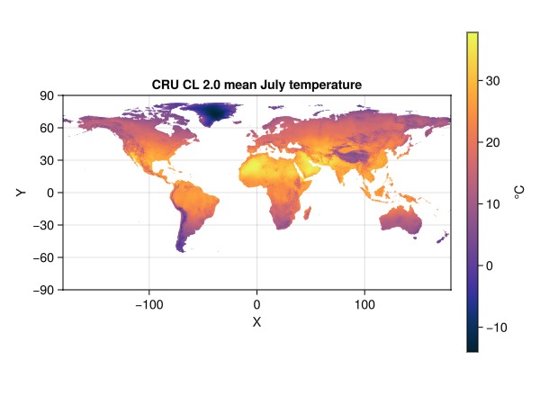

Regrid the raster onto HEALPix level 6

Regridding returns a Raster whose single dimension is Cells: the grid's cells, in the grid's order. That axis is what every selector below indexes.

grid = DGG.levelgrid(DGG.HEALPixSystem(), 6)
field = DGG.regrid(tavg; to = grid)

┌ 49152-element Raster{Union{Missing, Float32}, 1} tmp ┐
├──────────────────────────────────────────────────────┴────────── dims ┐
  ↓ Cells CellLookup(HEALPixSystem, level=6, ncells=49152, 1 windows)
├───────────────────────────────────────────────────────────── metadata ┤
  Metadata{Rasters.NCDsource} of Dict{String, Any} with 3 entries:
  "_FillValue" => NaN
  "units"      => "C"
  "long_name"  => "mean temperature"
├─────────────────────────────────────────────────────────────── raster ┤
  missingval: missing
  extent: Extent(Cells = (LevelIndex(6, 0), LevelIndex(6, 49151)),)
└───────────────────────────────────────────────────────────────────────┘
 LevelIndex(6, 0)        missing
 LevelIndex(6, 1)        missing
 ⋮                     
 LevelIndex(6, 49150)  26.4508
 LevelIndex(6, 49151)    missing

Average the field over every country

DGG.zonal selects cells once per country and applies the reduction. The default includes cells whose canonical centre lies in the country.

countries = NaturalEarth.naturalearth("admin_0_countries", 50)

FeatureCollection with 242 Features

percountry = parent(DGG.zonal(mean, field; of=countries.geometry, emptyval=NaN))

242-element Vector{AbstractFloat}:
  15.685734f0
  17.084665f0
  29.872763f0
  27.005611f0
  24.639389f0
 NaN
 NaN
  28.152153f0
  11.781299f0
 NaN
   ⋮
  18.018764f0
 NaN
  32.856735f0
  20.4494f0
  24.858145f0
 NaN
 NaN
 NaN
 NaN

At this resolution, small islands may have no selected land cell, and the source has no observations for some Antarctic regions. Those means are NaN; the ranking places them at the end and the map draws them grey.

ranked = sort(countries.NAME .=> round.(percountry; digits = 1); by = last)
last(filter(!isnan ∘ last, ranked), 5)

5-element Vector{Pair{String}}:
         "Saudi Arabia" => 33.2f0
           "Mauritania" => 33.8f0
                 "Iraq" => 34.0f0
 "United Arab Emirates" => 35.3f0
               "Kuwait" => 36.5f0

The five coldest:

first(ranked, 5)

5-element Vector{Pair{String}}:
   "Greenland" => -4.1f0
 "New Zealand" => 4.7f0
       "Chile" => 4.9f0
     "Lesotho" => 6.8f0
     "Iceland" => 7.8f0

crange = extrema(skipmissing(field))
fnan = Rasters.replace_missing(field, NaN)

fig = Figure(size = (900, 900))
ax1 = GeoAxis(fig[1, 1]; dest = "+proj=eqearth",
    title = "July mean temperature on HEALPix level 6",
    xgridcolor = (:black, 0.15), ygridcolor = (:black, 0.15))
dggpoly!(ax1, fnan; color = fnan, colormap = :thermal, colorrange = crange)
lines!(ax1, GeoMakie.coastlines(); color = (:black, 0.45), linewidth = 0.5)
Colorbar(fig[1, 2]; colormap = :thermal, colorrange = crange, label = "°C")
ax2 = GeoAxis(fig[2, 1]; dest = "+proj=eqearth",
    title = "mean July temperature per country",
    xgridcolor = (:black, 0.15), ygridcolor = (:black, 0.15))
poly!(ax2, countries.geometry; color = percountry, colormap = :thermal,
    colorrange = crange, strokecolor = (:black, 0.4), strokewidth = 0.4,
    nan_color = :lightgray)
Colorbar(fig[2, 2]; colormap = :thermal, colorrange = crange, label = "°C")
fig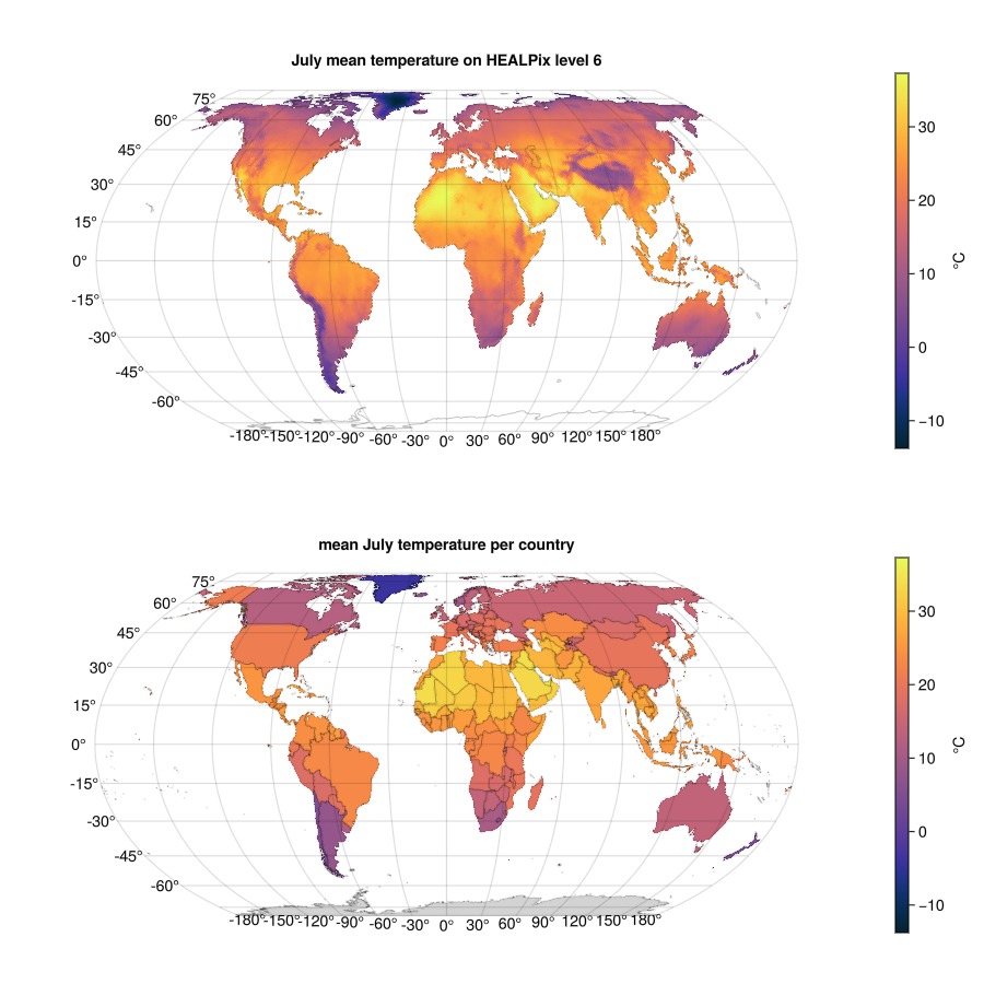

Whole cells approximate each country. boundary=:inside selects cells wholly within its boundary; boundary=:intersects includes any intersecting cell. These are membership rules, not fractional polygon-area weights.

Select the cells covering one region

The same selector on one state gives a Raster over the cells covering it.

states = NaturalEarth.naturalearth("admin_1_states_provinces", 50)
texas = states.geometry[findfirst(==("Texas"), states.name)]

tx = field[DGG.Cells(DGG.Covering(texas))]

┌ 95-element Raster{Union{Missing, Float32}, 1} tmp ┐
├───────────────────────────────────────────────────┴─────────── dims ┐
  ↓ Cells CellLookup(HEALPixSystem, level=6, ncells=95, 23 windows)
├─────────────────────────────────────────────────────────── metadata ┤
  Metadata{Rasters.NCDsource} of Dict{String, Any} with 3 entries:
  "_FillValue" => NaN
  "units"      => "C"
  "long_name"  => "mean temperature"
├───────────────────────────────────────────────────────────── raster ┤
  missingval: missing
  extent: Extent(Cells = (LevelIndex(6, 9297), LevelIndex(6, 32702)),)
└─────────────────────────────────────────────────────────────────────┘
 LevelIndex(6, 9297)   27.7831
 LevelIndex(6, 9299)   28.3511
 ⋮                     
 LevelIndex(6, 32701)  26.9735
 LevelIndex(6, 32702)  27.9242

DGG.zonal(mean, field; of=texas, emptyval=NaN)

28.035667f0

HEALPix cells have equal area, so the plain mean is area-weighted for this grid. On a system with unequal cells, weight by DGG.cell_area.(grid, DD.lookup(tx, DGG.Cells)).

Draw the covering cells of Texas

replace_missing turns the Gulf-coast cells into NaN, and dggpoly! leaves those undrawn.

txn = Rasters.replace_missing(tx, NaN)

fig = Figure(size = (760, 620))
ax = GeoAxis(fig[1, 1]; dest = "+proj=longlat +datum=WGS84",
    limits = ((-110.0, -91.0), (23.5, 39.0)), xticks = -108:2:-92,
    yticks = 24:2:38, xgridcolor = (:black, 0.15), ygridcolor = (:black, 0.15),
    title = "HEALPix level-6 cells covering Texas")
dggpoly!(ax, txn; color = txn, colormap = :thermal,
    strokecolor = (:white, 0.6), strokewidth = 0.5)
poly!(ax, texas; color = :transparent, strokecolor = :black, strokewidth = 2)
Colorbar(fig[1, 2]; colormap = :thermal, colorrange = extrema(skipmissing(tx)),
    label = "°C")
fig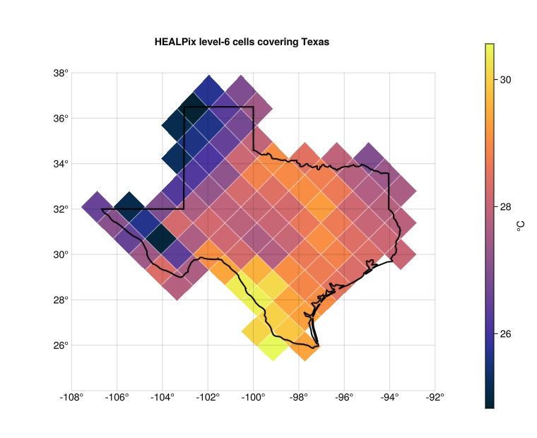

Narrow the selection by boundary rule

These boundary rules select progressively narrower sets of cells. A raster zonal tool commonly uses the centre-in-zone rule for its pixels.

rule	cells kept	spelling
Covering	a cell set containing the outline, possibly with an outer rim	field[Cells(Covering(geom))]
CentroidCovered	every cell whose centre is inside	field[Cells(CentroidCovered(geom))]
Within	every cell wholly inside the outline	field[Cells(Within(geom))]

CentroidCovered is the centre-in-zone rule the raster operations spell boundary=:center; see the raster APIs.

centred = field[DGG.Cells(DGG.CentroidCovered(texas))]
inside = field[DGG.Cells(DGG.Within(texas))]

┌ 41-element Raster{Union{Missing, Float32}, 1} tmp ┐
├───────────────────────────────────────────────────┴────────── dims ┐
  ↓ Cells CellLookup(HEALPixSystem, level=6, ncells=41, 9 windows)
├────────────────────────────────────────────────────────── metadata ┤
  Metadata{Rasters.NCDsource} of Dict{String, Any} with 3 entries:
  "_FillValue" => NaN
  "units"      => "C"
  "long_name"  => "mean temperature"
├──────────────────────────────────────────────────────────── raster ┤
  missingval: missing
  extent: Extent(Cells = (LevelIndex(6, 9302), LevelIndex(6, 32698)),)
└────────────────────────────────────────────────────────────────────┘
 LevelIndex(6, 9302)   26.4074
 LevelIndex(6, 9303)   27.6447
 ⋮                     
 LevelIndex(6, 32697)  28.6878
 LevelIndex(6, 32698)  29.0481

mean(skipmissing(tx)), mean(skipmissing(centred)), mean(skipmissing(inside))

(27.930677f0, 28.035667f0, 28.112486f0)

The means differ because boundary cells change which ground contributes to the statistic.

Read the cell holding a point

DD.Contains takes a position in degrees and selects the cell holding it. Austin sits at 97.74° W, 30.27° N.

field[DGG.Cells(DD.Contains((-97.74, 30.27)))]

28.686125f0

Run the same statistic on another system

The same selectors work with another grid system. Here levelfor chooses an IGEO7 level with cells approximately 100 km across:

igeo7 = DGG.IGeo7System()
level = DGG.levelfor(igeo7, 100_000)

4

field7 = DGG.regrid(tavg; to = DGG.levelgrid(igeo7, level))

┌ 24012-element Raster{Union{Missing, Float32}, 1} tmp ┐
├──────────────────────────────────────────────────────┴──────── dims ┐
  ↓ Cells CellLookup(IGeo7System, level=4, ncells=24012, 1 windows)
├─────────────────────────────────────────────────────────── metadata ┤
  Metadata{Rasters.NCDsource} of Dict{String, Any} with 3 entries:
  "_FillValue" => NaN
  "units"      => "C"
  "long_name"  => "mean temperature"
├───────────────────────────────────────────────────────────── raster ┤
  missingval: missing
  extent: Extent(Cells = (Z7Cell("000000"), Z7Cell("116666")),)
└─────────────────────────────────────────────────────────────────────┘
 Z7Cell("000000")    missing
 Z7Cell("000001")  15.7544
 ⋮                 
 Z7Cell("116665")    missing
 Z7Cell("116666")    missing

mean(skipmissing(field7[DGG.Cells(DGG.Covering(texas))]))

27.864496f0

The width of the covering rim depends on the grid's refinement scheme; Multi-order coverage shows where that width comes from.

Without the DimArray

CellVector exposes the grid as a vector of cell ids. The two functions below show the index operations used by Covering and Contains on the Cells axis:

cells = DGG.CellVector(grid)
DGG.covering_indices(cells, texas)

95-element Vector{Int64}:
  9298
  9300
  9301
  9302
  9303
  9304
  9306
  9308
  9309
  9310
     ⋮
 32695
 32696
 32697
 32698
 32699
 32700
 32701
 32702
 32703

DGG.localindex(cells, -97.74, 30.27)

32679

Extract values and labelled slices

Extraction returns named-tuple rows, including local cell-axis positions.

texas_rows = DGG.extract(field, texas; index=true, skipmissing=true)
first(texas_rows, 5)

5-element Vector{@NamedTuple{geometry::Tuple{Float64, Float64}, index::Int64, tmp::Float32}}:
 (geometry = (-101.95312500000001, 30.000000000000004), index = 9302, tmp = 29.08659)
 (geometry = (-103.35937499999999, 30.000000000000004), index = 9303, tmp = 26.407373)
 (geometry = (-102.65625000000001, 30.69158768492234), index = 9304, tmp = 27.644695)
 (geometry = (-104.06250000000003, 30.69158768492234), index = 9309, tmp = 24.913681)
 (geometry = (-103.35937499999999, 31.388166464348547), index = 9310, tmp = 28.218676)

---

This page was generated using Literate.jl.