Creating Geometry
In this tutorial, we're going to build some basic 2D geometry. This follows the Simple Features hierarchy for geospatial geometry:
Install the packages used in this tutorial:
using Pkg
Pkg.add(["GeoInterface", "GeometryOps",
        "CoordinateTransformations",
"CairoMakie", "GeoMakie"])# Geospatial packages from Julia
import GeoInterface as GI
import GeometryOps as GO
# Coordinate transformation and projection
import CoordinateTransformations
# Plotting
using CairoMakie
using GeoMakieCreate Points and MultiPoints
Let's start by making a single Point.
point = GI.Point(0, 0)Point{false, false}((0, 0))Now, let's plot our point.
fig, ax, plt = plot(point)
Let's create a set of points, and have a bit more fun with plotting.
xs = [-5, 0, 5, 0]
ys = [0, -5, 0, 5]

points = GI.Point.(xs, ys)

plot!(ax, points; marker = '✈', markersize = 30)
fig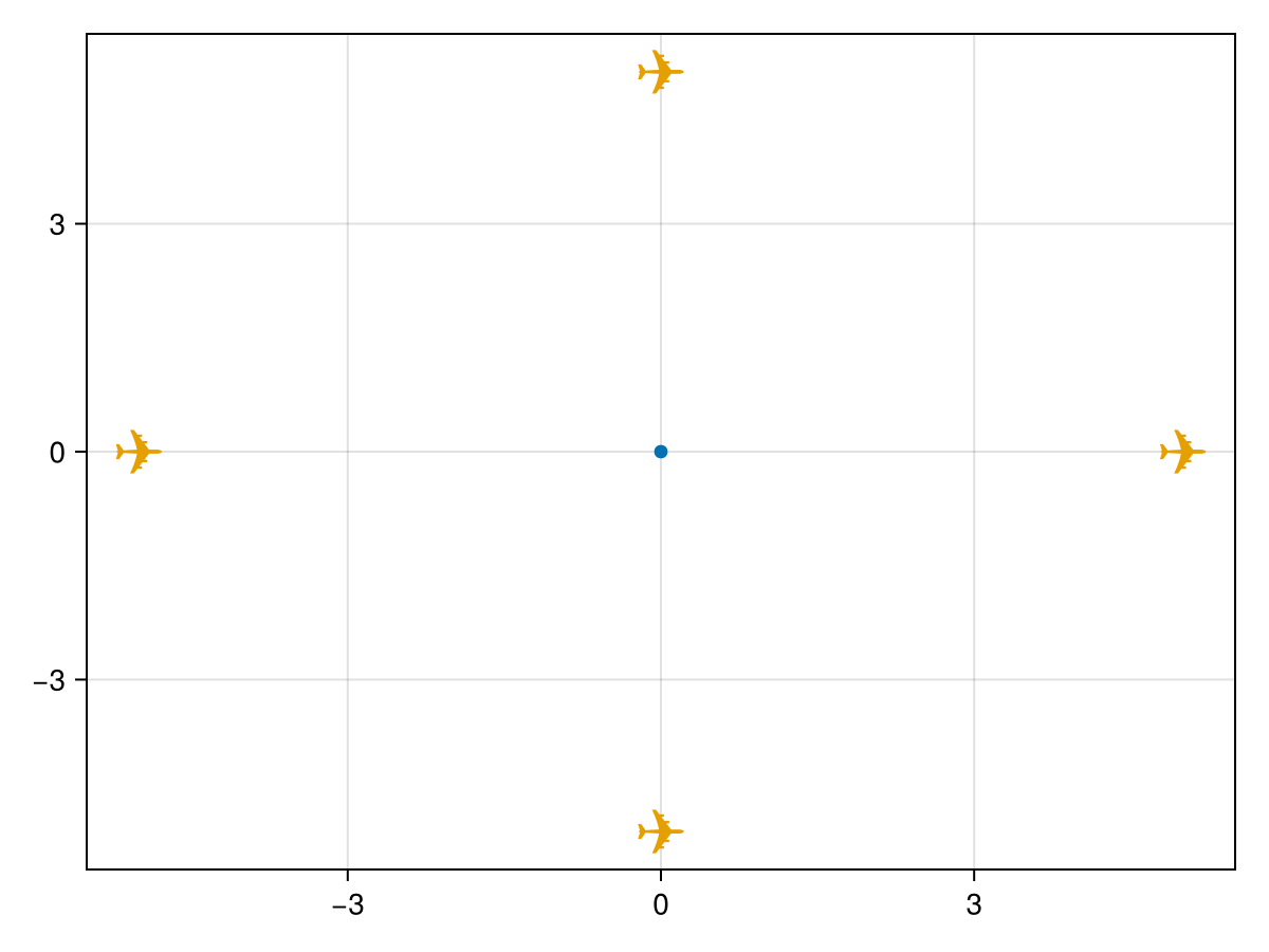
Points can be combined into a single MultiPoint geometry.
xs = [-5, -5, 5, 5]
ys = [-5, 5, 5, -5]

# zip: Create (x, y) coordinates (tuples)
# GI.Point: Turn each coordinate pair into special Point geometries
# GI.MultiPoint: Wrap all Points into a single MultiPoint geometry object
multipoint = GI.MultiPoint(GI.Point.(xs, ys));
# TODO: GeoInterfaceMakie.jl can't plot multipoints due to breaking changes
# in Makie.jl.  We should fix that.
plot!(ax, multipoint.geom; marker = '☁', markersize = 30)
fig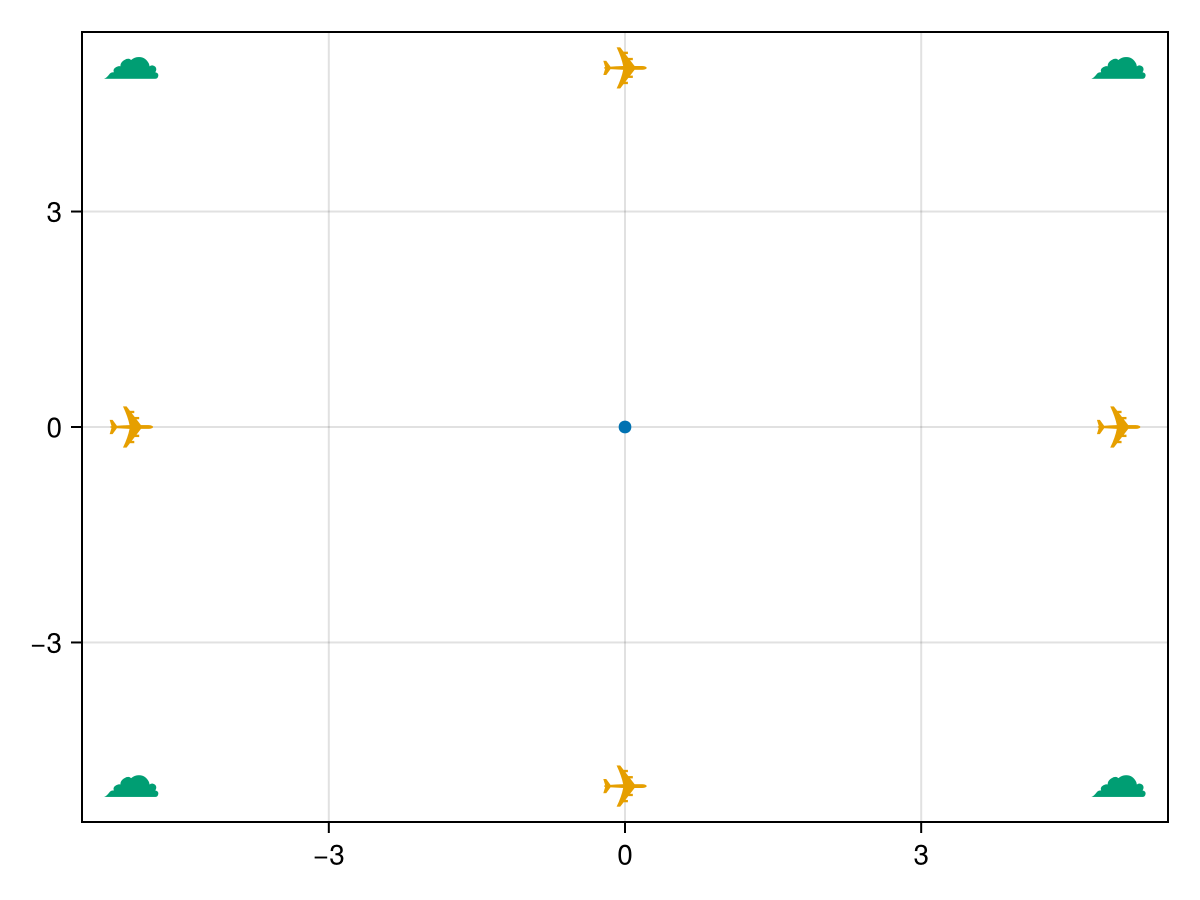
Connecting points into lines
Let's create a LineString connecting two points.
p1 = GI.Point.(-5, 0)
p2 = GI.Point.(5, 0)
line = GI.LineString([p1, p2])
plot!(ax, line; color = :red)
fig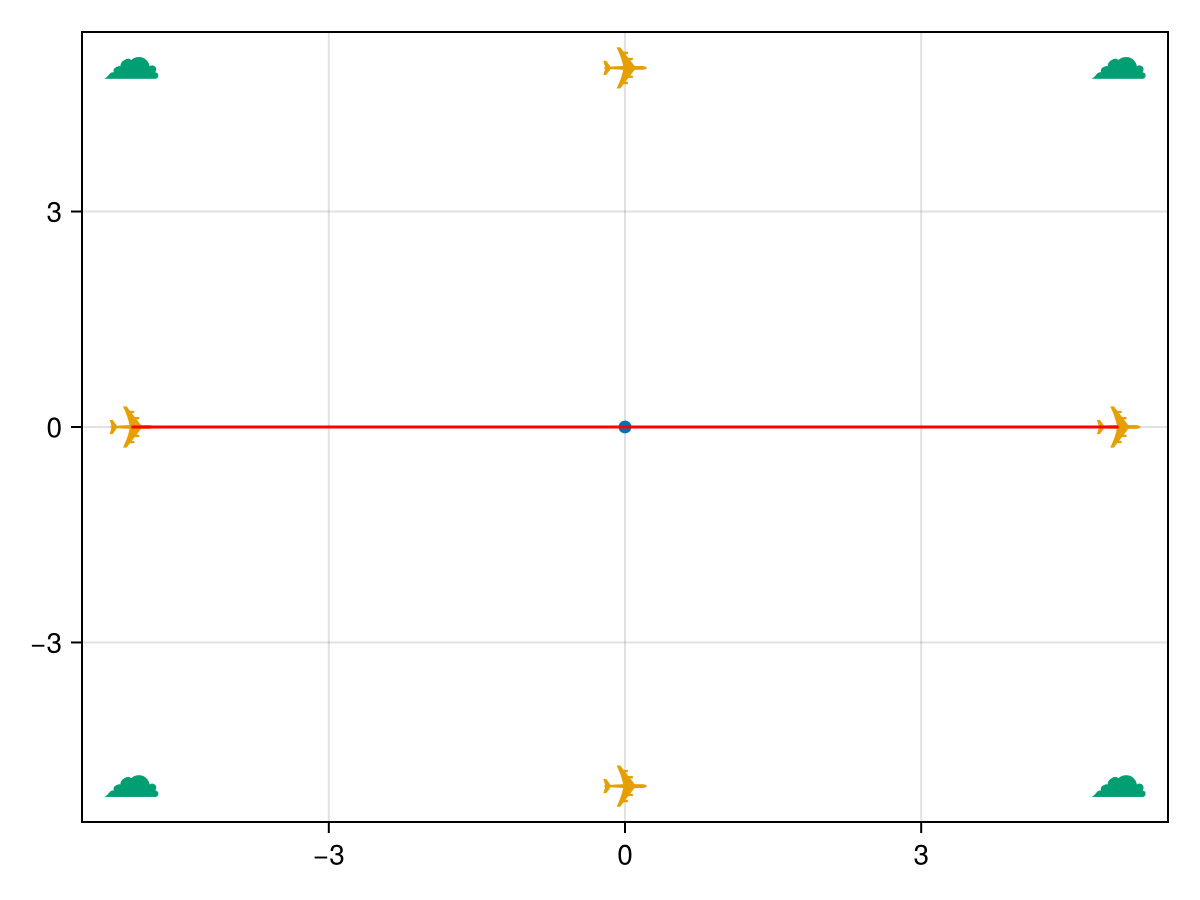
Now, let's create a line connecting multiple points (i.e. a LineString). This time we get a bit more fancy with point creation.
r = 2
k = 10
ϴs = 0:0.01:2pi
xs = r .* (k + 1) .* cos.(ϴs) .- r .* cos.((k + 1) .* ϴs)
ys = r .* (k + 1) .* sin.(ϴs) .- r .* sin.((k + 1) .* ϴs)

lines = GI.LineString(GI.Point.(xs, ys))

plot!(ax, lines; linewidth = 5)
fig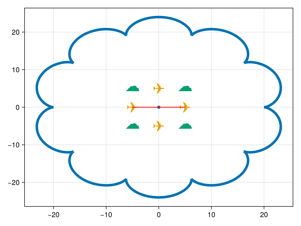
Building polygons and multipolygons
We can also create a single LinearRing trait, the building block of a polygon. A LinearRing is simply a LineString with the same beginning and endpoint, i.e., an arbitrary closed shape composed of point pairs.
A LinearRing is composed of a series of points.
ring1 = GI.LinearRing(GI.getpoint(lines));GeoInterface.Wrappers.LinearRing{false, false}([Point((20.0, 0.0)), … (627) … , Point((20.001115954499138, -1.4219350464667047e-5))])Now, let's make the LinearRing into a Polygon.
# Polygon fills the interior of a LinearRing, turning it into a solid shape
polygon1 = GI.Polygon([ring1]);
GeoInterface.Wrappers.Polygon{false, false}([GeoInterface.Wrappers.LinearRing([Point((20.0, 0.0)), … (627) … , Point((20.001115954499138, -1.4219350464667047e-5))])])Now, we can use GeometryOps and CoordinateTransformations to shift polygon1 up, to avoid plotting over our earlier results. This is done through the GeometryOps.transform function.
xoffset = 0.
yoffset = 50.
f = CoordinateTransformations.Translation(xoffset, yoffset)
polygon1 = GO.transform(f, polygon1)
plot!(polygon1)
fig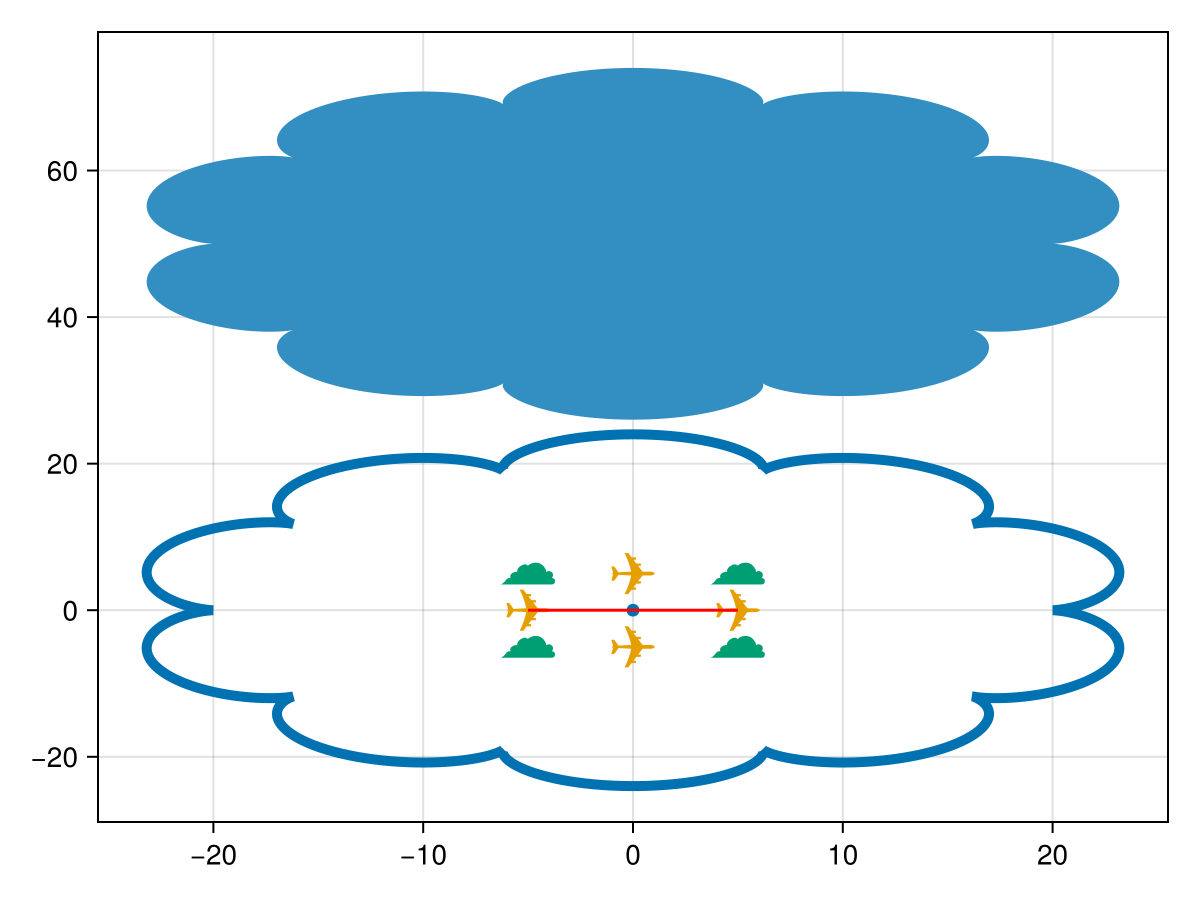
Polygons can contain "holes". The first LinearRing in a polygon is the exterior, and all subsequent LinearRings are treated as holes in the leading LinearRing.
GeoInterface offers the GI.getexterior(poly) and GI.gethole(poly) methods to get the exterior ring and an iterable of holes, respectively.
hole = GI.LinearRing(GI.getpoint(multipoint))
polygon2 = GI.Polygon([ring1, hole])
GeoInterface.Wrappers.Polygon{false, false}([GeoInterface.Wrappers.LinearRing([Point((20.0, 0.0)), … (627) … , Point((20.001115954499138, -1.4219350464667047e-5))]), GeoInterface.Wrappers.LinearRing([Point((-5, -5)), … (2) … , Point((5, -5))])])Shift polygon2 to the right, to avoid plotting over our earlier results.
xoffset = 50.
yoffset = 0.
f = CoordinateTransformations.Translation(xoffset, yoffset)
polygon2 = GO.transform(f, polygon2)
plot!(polygon2)
fig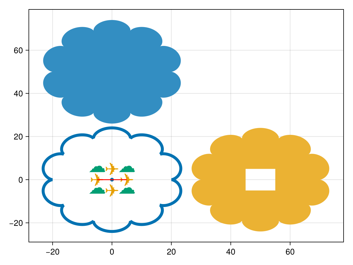
Similar to Points with MultiPoints, Polygons can also be grouped together as a MultiPolygon.
# Create a simple circle with a radius of 5
r = 5
xs = cos.(reverse(ϴs)) .* r .+ xoffset
ys = sin.(reverse(ϴs)) .* r .+ yoffset
ring2 =  GI.LinearRing(GI.Point.(xs, ys))
polygon3 = GI.Polygon([ring2])

# Group polygon2 (our shape with the square hole) and polygon3 (our circle) together into a MultiPolygon
multipolygon = GI.MultiPolygon([polygon2, polygon3])
GeoInterface.Wrappers.MultiPolygon{false, false}([GeoInterface.Wrappers.Polygon([GeoInterface.Wrappers.LinearRing([[70.0, 0.0], … (627) … , [70.00111595449914, -1.4219350464667047e-5]]), GeoInterface.Wrappers.LinearRing([[45.0, -5.0], … (2) … , [55.0, -5.0]])]), GeoInterface.Wrappers.Polygon([GeoInterface.Wrappers.LinearRing([Point((54.999974634566875, -0.01592650896568995)), … (627) … , Point((55.0, 0.0))])])])Shift multipolygon up, to avoid plotting over our earlier results.
xoffset = 0.
yoffset = 50.
f = CoordinateTransformations.Translation(xoffset, yoffset)
multipolygon = GO.transform(f, multipolygon)
plot!(multipolygon)
fig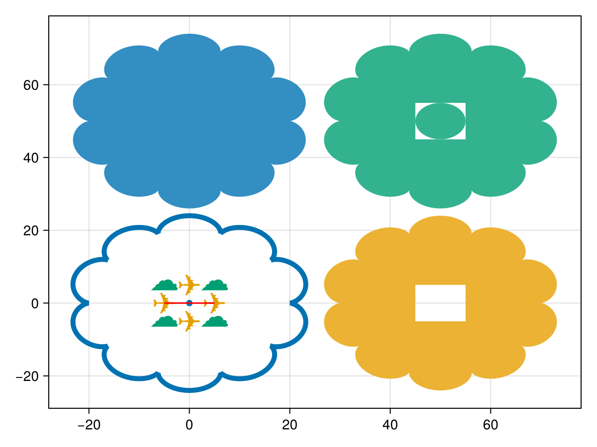
Great, now we can make Points, MultiPoints, Lines, LineStrings, Polygons (with holes), and MultiPolygons and modify them using [CoordinateTransformations] and [GeometryOps].