Geospatial Geometry

In this tutorial, we're going to:

1. Plot geometries on a map using GeoMakie and coordinate reference system (CRS)

2. Create geospatial geometries with embedded coordinate reference system information

3. Assign attributes to geospatial geometries

4. Save geospatial geometries to common geospatial file formats

5. Introduce Geodesic Paths

Install the packages used in this tutorial:

using Pkg
Pkg.add(["GeoInterface", "GeometryOps", "GeoFormatTypes", 
        "GeoJSON", "GeoParquet", "GeoDataFrames",
        "CoordinateTransformations", "Proj", "DataFrames", 
        "CairoMakie", "GeoMakie", "Shapefile"])

# Geospatial packages
import GeoInterface as GI
import GeometryOps as GO
import GeoFormatTypes as GFT
# Coordinate transformation and projection
import CoordinateTransformations
import Proj
# Plotting
using CairoMakie
using GeoMakie
# Data loading
using GeoDataFrames, DataFrames
import GeoParquet, GeoJSON, Shapefile # activate native IO packages

Plot geometries on a map using GeoMakie and coordinate reference system (CRS)

In geospatial sciences we often have data in one Coordinate Reference System (CRS) (source) and would like to display it in different (destination) CRS. GeoMakie allows us to do this by automatically projecting from source to destination CRS.

Here, our source CRS is common geographic (i.e. coordinates of latitude and longitude), WGS84.

source_crs1 = GFT.EPSG(4326)

EPSG:4326

Now let's pick a destination CRS for displaying our map. Here we'll pick natearth2.

destination_crs = "+proj=natearth2"

"+proj=natearth2"

Let's add land area for context. First, download and open the Natural Earth global land polygons at 110 m resolution. GeoMakie ships with this particular dataset, so we will access it from there. Note that this will be a path on your local machine, so you could easily point it to any other .geojson file you have.

land_geojson_path = GeoMakie.assetpath("ne_110m_land.geojson")

"/home/runner/.julia/packages/GeoMakie/QcBwP/assets/ne_110m_land.geojson"

Note

Natural Earth has lots of other datasets, and there is a Julia package that provides an interface to it called NaturalEarth.jl.

Read this dataset in as a GeoJSON.FeatureCollection.

land_features = GeoDataFrames.read(land_geojson_path)

127×4 DataFrame

Row	min_zoom	geometry	scalerank	featurecla
	Union…	Polygon…	Int64	String
1	1	2D Polygon	1	Land
2	1	2D Polygon	1	Land
3	0	2D Polygon	1	Land
4	1	2D Polygon	1	Land
5	1	2D Polygon	1	Land
6	1	2D Polygon	1	Land
7	1	2D Polygon	1	Land
8	0	2D Polygon	0	Land
9	0	2D Polygon	0	Land
10	0.5	2D Polygon	0	Land
11	0.5	2D Polygon	0	Land
12	0	2D Polygon	0	Land
13	0	2D Polygon	0	Land
14	0	2D Polygon	0	Land
15	1	2D Polygon	1	Land
16	0.5	2D Polygon	0	Land
17	1.5	2D Polygon	0	Land
18	1.5	2D Polygon	1	Land
19	1.5	2D Polygon	1	Land
20	1	2D Polygon	1	Land
21	0	2D Polygon	0	Land
22	0	2D Polygon	0	Land
23	1.5	2D Polygon	1	Land
24	1.5	2D Polygon	1	Land
25	1	2D Polygon	1	Land
26	1.5	2D Polygon	1	Land
27	1	2D Polygon	1	Land
28	1	2D Polygon	1	Land
29	1	2D Polygon	1	Land
30	1	2D Polygon	1	Land
31	1.5	2D Polygon	1	Land
32	0	2D Polygon	0	Land
33	1.5	2D Polygon	1	Land
34	1	2D Polygon	1	Land
35	1	2D Polygon	1	Land
36	1.5	2D Polygon	1	Land
37	1	2D Polygon	1	Land
38	1.5	2D Polygon	1	Land
39	0	2D Polygon	0	Land
40	0	2D Polygon	0	Land
41	1	2D Polygon	1	Land
42	0	2D Polygon	0	Land
43	0	2D Polygon	0	Land
44	0	2D Polygon	0	Land
45	1	2D Polygon	1	Land
46	1	2D Polygon	0	Land
47	1	2D Polygon	1	Land
48	1	2D Polygon	1	Land
49	1	2D Polygon	1	Land
50	0	2D Polygon	0	Land
51	1.5	2D Polygon	1	Land
52	0	2D Polygon	0	Land
53	1	2D Polygon	1	Land
54	1	2D Polygon	1	Land
55	0	2D Polygon	0	Land
56	1	2D Polygon	1	Land
57	0.5	2D Polygon	0	Land
58	1.5	2D Polygon	0	Land
59	1.5	2D Polygon	0	Land
60	1	2D Polygon	0	Land
61	1.5	2D Polygon	0	Land
62	0	2D Polygon	0	Land
63	1	2D Polygon	0	Land
64	1	2D Polygon	1	Land
65	1.5	2D Polygon	0	Land
66	1.5	2D Polygon	0	Land
67	1.5	2D Polygon	1	Land
68	1	2D Polygon	1	Land
69	1	2D Polygon	1	Land
70	1	2D Polygon	1	Land
71	1	2D Polygon	1	Land
72	0	2D Polygon	0	Land
73	1	2D Polygon	1	Land
74	0	2D Polygon	0	Land
75	1	2D Polygon	0	Land
76	1	2D Polygon	0	Land
77	1	2D Polygon	1	Land
78	0	2D Polygon	0	Land
79	1	2D Polygon	1	Land
80	0	2D Polygon	0	Land
81	0	2D Polygon	0	Land
82	1	2D Polygon	1	Land
83	1	2D Polygon	1	Land
84	0	2D Polygon	0	Land
85	1.5	2D Polygon	0	Land
86	1.5	2D Polygon	0	Land
87	1.5	2D Polygon	0	Land
88	1.5	2D Polygon	1	Land
89	0.5	2D Polygon	1	Land
90	0	2D Polygon	0	Land
91	1	2D Polygon	0	Land
92	0	2D Polygon	0	Land
93	1.5	2D Polygon	1	Land
94	1	2D Polygon	0	Land
95	0	2D Polygon	0	Land
96	0	2D Polygon	0	Land
97	0	2D Polygon	0	Land
98	1.5	2D Polygon	0	Land
99	1	2D Polygon	0	Land
100	0	2D Polygon	0	Land
101	0	2D Polygon	0	Land
102	1	2D Polygon	0	Land
103	0.5	2D Polygon	0	Land
104	0	2D Polygon	0	Land
105	1	2D Polygon	0	Land
106	1.5	2D Polygon	1	Land
107	0	2D Polygon	0	Land
108	0	2D Polygon	0	Land
109	0	2D Polygon	0	Land
110	0	2D Polygon	0	Land
111	0	2D Polygon	0	Land
112	0.5	2D Polygon	1	Land
113	0	2D Polygon	0	Land
114	1.5	2D Polygon	1	Land
115	1	2D Polygon	1	Land
116	1	2D Polygon	1	Land
117	1.5	2D Polygon	1	Land
118	1	2D Polygon	1	Land
119	0.5	2D Polygon	1	Land
120	0.5	2D Polygon	0	Land
121	0	2D Polygon	0	Land
122	0	2D Polygon	0	Land
123	1	2D Polygon	1	Land
124	0	2D Polygon	0	Land
125	0	2D Polygon	0	Land
126	0	2D Polygon	0	Land
127	0	2D Polygon	0	Land

We then need to create a figure with a GeoAxis that can handle the projection between source and destination CRS. For GeoMakie, source is the CRS of the input and dest is the CRS you want to visualize in.

fig = Figure(size=(1000, 500));
ga = GeoAxis(
    fig[1, 1];
    source = source_crs1,
    dest = destination_crs,
    xticklabelsvisible = false,
    yticklabelsvisible = false,
);

Plot land for context.

poly!(ga, land_features; color=:black)
fig

Now let's plot a Polygon like before, but this time with a CRS that differs from our source data.

function ring(radius)
    ϴ = 0:0.01:2π
	points = @. GI.Point(50 + radius * cos(ϴ), 50 + radius * sin(ϴ))
	return GI.LinearRing(points)
end

function spiro(a = 22, b = 2, k = 11)
    ϴ = 0:0.01:2π
    points = @. GI.Point(
        50 + a*cos(ϴ) - b*cos(k*ϴ),
        50 + a*sin(ϴ) - b*sin(k*ϴ)
    )
    return GI.LinearRing(points)
end


multipolygon = GI.MultiPolygon([
    GI.Polygon([spiro(), ring(8)]),
    GI.Polygon([ring(4)])
])

plot!(multipolygon; color = :green)
fig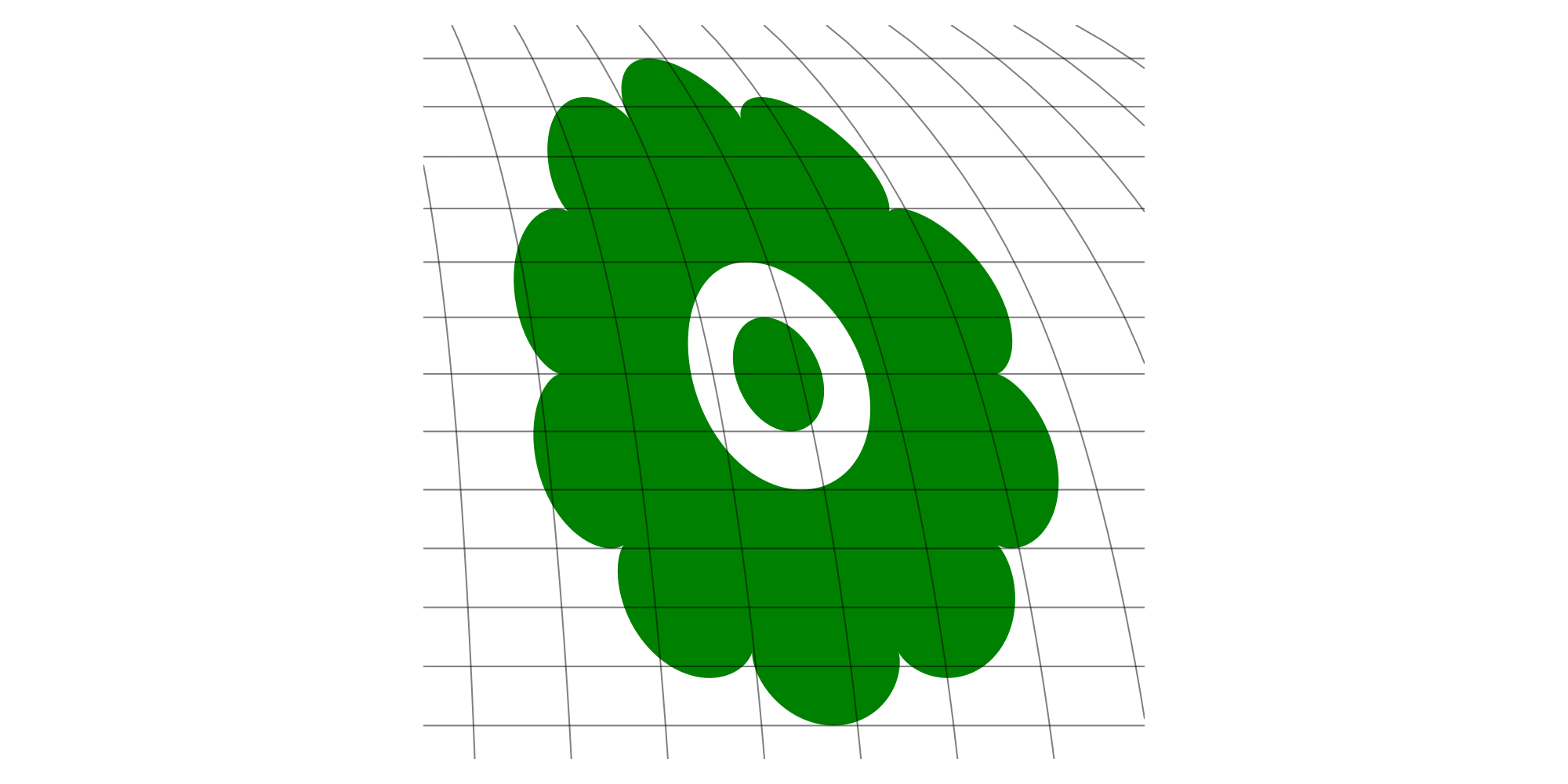

But what if we want to plot geometries with a different source CRS on the same figure?

To show how to do this let's create a geometry with coordinates in UTM (Universal Transverse Mercator) zone 10N EPSG:32610.

source_crs2 = GFT.EPSG(32610)

EPSG:32610

Create a polygon (we're working in meters now, not latitude and longitude)

rs = 1000000;
ϴs = 0:0.01:2pi;
xs = rs .* cos.(ϴs).^3 .+ 500000;
ys = rs .* sin.(ϴs) .^ 3 .+ 5000000;
DisplayAs.setcontext(y, :compact => true, :displaysize => (10, 40),) # hide

Now create a LinearRing from Points

ring3 = GI.LinearRing(GI.Point.(xs, ys))

GeoInterface.Wrappers.LinearRing{false, false}([Point((1.5e6, 5.0e6)), … (627) … , Point((1.499984780817334e6, 4.999999967681458e6))])

Now create a Polygon from the LineRing

polygon3 = GI.Polygon([ring3])

GeoInterface.Wrappers.Polygon{false, false}([GeoInterface.Wrappers.LinearRing([Point((1.5e6, 5.0e6)), … (627) … , Point((1.499984780817334e6, 4.999999967681458e6))])])

Now plot on the existing GeoAxis.

Note

The keyword argument source is used to specify the source CRS of that particular plot, when plotting on an existing GeoAxis.

plot!(ga,polygon3; color=:red, source = source_crs2)
fig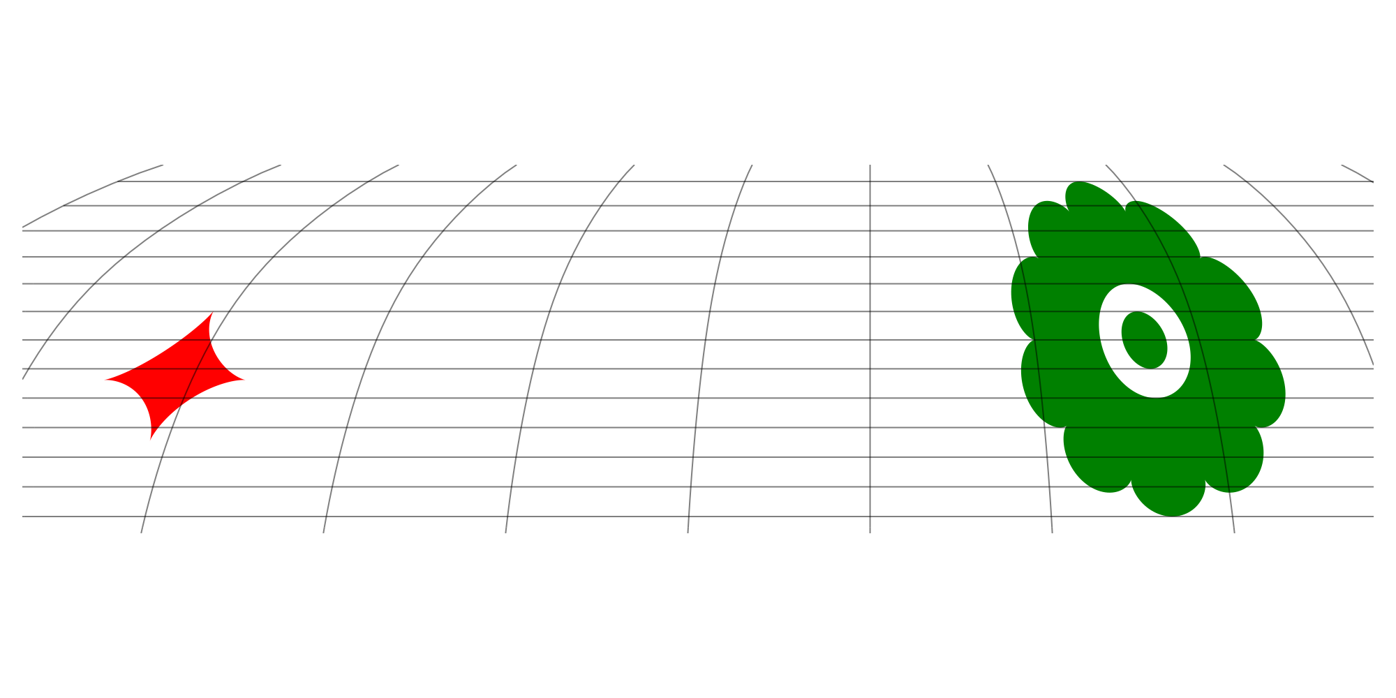

Create geospatial geometries with embedded coordinate reference system information

Great, we can make geometries and plot them on a map... now let's export the data to common geospatial data formats. To do this we now need to create geometries with embedded CRS information, making it a geospatial geometry. All that's needed is to include ; crs = crs as a keyword argument when constructing the geometry.

Let's do this for a new Polygon

rs = 3;
ks = 7;
ϴs = 0:0.01:2pi;
xs = rs .* (ks + 1) .* cos.(ϴs) .- rs .* cos.((ks + 1) .* ϴs);
ys = rs .* (ks + 1) .* sin.(ϴs) .- rs .* sin.((ks + 1) .* ϴs);
ring4 = GI.LinearRing(tuple.(xs, ys))

GeoInterface.Wrappers.LinearRing{false, false}([(21.0, 0.0), … (627) … , (21.00085222666982, -8.14404531208901e-6)])

But this time when we create the Polygon we need to specify the CRS at the time of creation, associating that metadata with the geometry.

geopoly1 = GI.Polygon([ring4], crs = source_crs1)

GeoInterface.Wrappers.Polygon{false, false}([GeoInterface.Wrappers.LinearRing([(21.0, 0.0), … (627) … , (21.00085222666982, -8.14404531208901e-6)])], crs = "EPSG:4326")

Note

It is good practice to only include CRS information with the highest-level geometry. Not doing so can sometimes bloat the memory footprint of the geometry. CRS information can be included at the individual Point level but is discouraged.

And let's create a second Polygon by shifting the first using CoordinateTransformations

xoffset = 20.
yoffset = -25.
f = CoordinateTransformations.Translation(xoffset, yoffset)
geopoly2 = GO.transform(f, geopoly1)

GeoInterface.Wrappers.Polygon{false, false}([GeoInterface.Wrappers.LinearRing([[41.0, -25.0], … (627) … , [41.00085222666982, -25.000008144045314]], crs = "EPSG:4326")], crs = "EPSG:4326")

Creating a table with attributes and geometry

Typically, you'll also want to include attributes with your geometries. Attributes are simply data that are attributed to each geometry. The easiest way to do this is to create a table with a :geometry column. Let's do this using DataFrames.

df = DataFrame(geometry = [geopoly1, geopoly2])

2×1 DataFrame

Row	geometry
	Polygon…
1	GeoInterface.Wrappers.Polygon([GeoInterface.Wrappers.LinearRing([(21.0,0.0),…(627)…,(21.00085222666982,-8.14404531208901e-6)])])
2	GeoInterface.Wrappers.Polygon([GeoInterface.Wrappers.LinearRing([[41.0,-25.0],…(627)…,[41.00085222666982,-25.000008144045314]])])

Now let's add a couple of attributes to the geometries by adding new columns to our existing data frame.

df.id = ["a", "b"]
df.name = ["polygon 1", "polygon 2"]
df

2×3 DataFrame

Row	geometry	id	name
	Polygon…	String	String
1	GeoInterface.Wrappers.Polygon([GeoInterface.Wrappers.LinearRing([(21.0,0.0),…(627)…,(21.00085222666982,-8.14404531208901e-6)])])	a	polygon 1
2	GeoInterface.Wrappers.Polygon([GeoInterface.Wrappers.LinearRing([[41.0,-25.0],…(627)…,[41.00085222666982,-25.000008144045314]])])	b	polygon 2

Saving your geospatial data

There are Julia packages for most commonly used geographic data formats. Below, we show how to export that data to each of these.

In general, GeoDataFrames is recomended as the default way to write data to your desired format. This package uses the GDAL library under the hood which supports writing to nearly all geospatial formats.

Writing to gpkg:

GeoDataFrames.write("shapes.gpkg", df)

"shapes.gpkg"

Writing to GeoJSON:

GeoDataFrames.write("file.geojson", df)

"file.geojson"

View the GeoDataFrames documentation for all recognized file extensions.

Geodesic paths

Geodesic paths are paths computed on an ellipsoid, as opposed to a plane. The geodesic is the shortest path between two points measured along the Earth's curved surface. Because the surface is curved, that shortest path appears as a curve (not a straight line) when drawn on a flat map.

Here, we use the segmentize function to add vertices along the geodesic between two points, so the line follows Earth's curved surface instead of a straight line.

# Two points in (longitude, latitude) order: Houston (IAH) and Amsterdam (AMS).
# Geodesic methods assume lon/lat input.
IAH = (-95.358421, 29.749907)
AMS = (4.897070, 52.377956)

# Draw coastlines for geographic context
fig, ga, _cp = lines(GeoMakie.coastlines(); axis = (; type = GeoAxis))

# Create our line along the Earth, accounting for curvature
lines!(ga, GO.segmentize(GO.Geodesic(), GI.LineString([IAH, AMS]); max_distance = 100_000))
fig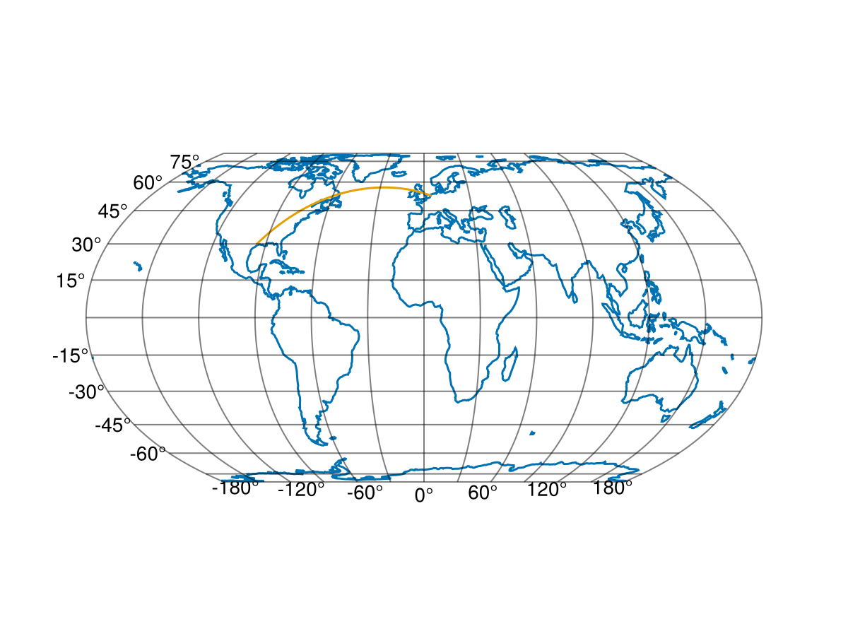

And there we go, you can now create mapped geometries from scratch, manipulate them, plot them on a map, and save them in multiple geospatial data formats, as well as create geodesic paths.